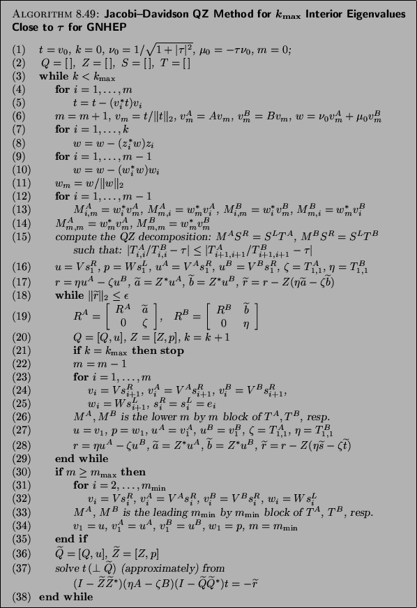
The Jacobi-Davidson algorithm is given in Algorithm 8.1. This
algorithm attempts to compute the generalized Schur pairs
![]() , for which the ratio
, for which the ratio ![]() is closest
to a specified target value
is closest
to a specified target value ![]() in the complex plane.
The algorithm includes restart in order to limit the dimension
of the search space, and deflation with already converged left and right
Schur vectors.
in the complex plane.
The algorithm includes restart in order to limit the dimension
of the search space, and deflation with already converged left and right
Schur vectors.
To apply this algorithm we need to specify a starting
vector ![]() , a tolerance
, a tolerance ![]() , a target value
, a target value ![]() , and a
number
, and a
number ![]() that specifies how many eigenpairs near
that specifies how many eigenpairs near ![]() should be computed. The value of
should be computed. The value of ![]() specifies the maximum
dimension of the search subspace. If it is exceeded then a restart
takes place with a subspace of dimension
specifies the maximum
dimension of the search subspace. If it is exceeded then a restart
takes place with a subspace of dimension ![]() .
.
On completion the ![]() generalized eigenvalues close to
generalized eigenvalues close to ![]() are delivered, and the corresponding reduced Schur form
are delivered, and the corresponding reduced Schur form ![]() ,
,
![]() , where
, where ![]() and
and ![]() are
are ![]() by
by ![]() orthogonal
and
orthogonal
and ![]() ,
, ![]() are
are ![]() by
by ![]() upper triangular.
The generalized eigenvalues are the on-diagonals of
upper triangular.
The generalized eigenvalues are the on-diagonals of ![]() and
and ![]() .
The computed form
satisfies
.
The computed form
satisfies
![]() ,
,
![]() ,
where
,
where ![]() is the
is the ![]() th column of
th column of ![]() .
.
The accuracy of the computed reduced Schur form depends on the
distance between the target value ![]() and the eigenvalue
and the eigenvalue
![]() .
If we neglect terms of
order machine precision and of order
.
If we neglect terms of
order machine precision and of order ![]() , then we have
that
, then we have
that
![]() ,
,
![]() ,
where the constants
,
where the constants
![]() and
and ![]() are given by
are given by
We will now explain the successive main phases of the algorithm.
We expand the subspaces ![]() ,
, ![]() ,
, ![]() , and
, and ![]() .
.
![]() denotes the matrix with the current basis vectors
denotes the matrix with the current basis vectors ![]() for
the search subspace as its columns. The other matrices are defined in
a similar obvious way.
for
the search subspace as its columns. The other matrices are defined in
a similar obvious way.
Note that the scalars ![]() can also be computed from
the scalars
can also be computed from
the scalars ![]() , and the orthogonalization constants
of
, and the orthogonalization constants
of ![]() in step (10).
in step (10).
The QZ decomposition for the pair ![]() of
of ![]() by
by ![]() matrices can be computed by a suitable
routine for dense matrix pencils from LAPACK.
matrices can be computed by a suitable
routine for dense matrix pencils from LAPACK.
We have
chosen to compute the generalized Petrov pairs, which makes the algorithm
suitable for computing ![]() interior generalized eigenvalues of
interior generalized eigenvalues of
![]() , for which
, for which ![]() is
close to a specified
is
close to a specified ![]() .
.
For algorithms for reordering the generalized Schur form, see [448,449,171].
Detection of all wanted eigenvalues cannot be guaranteed; see note (13)
for Algorithm 4.17 (p. ![]() ).
).
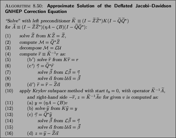
Of course, the correction equation can be solved by any
suitable process, for instance, a preconditioned Krylov subspace
method that is designed to solve unsymmetric systems. However, because
of the different projections, we always need a preconditioner (which may
be the identity operator if nothing else is available) that is deflated
by the same skew projections so that we obtain a mapping between
![]() and itself.
Because of the occurrence of
and itself.
Because of the occurrence of ![]() and
and ![]() , one
has to be
careful with the usage of preconditioners for the matrix
, one
has to be
careful with the usage of preconditioners for the matrix
![]() .
The inclusion of preconditioners can be done as in
Algorithm 8.2. Make sure that the starting vector
.
The inclusion of preconditioners can be done as in
Algorithm 8.2. Make sure that the starting vector ![]() for an iterative solver satisfies the orthogonality constraints
for an iterative solver satisfies the orthogonality constraints
![]() . Note
that significant savings per step
can be made in Algorithm 8.2 if
. Note
that significant savings per step
can be made in Algorithm 8.2 if ![]() is kept the same for a (few) Jacobi-Davidson iterations. In that case
columns of
is kept the same for a (few) Jacobi-Davidson iterations. In that case
columns of ![]() can be saved from previous steps. Also the matrix
can be saved from previous steps. Also the matrix
![]() can be updated from previous steps, as well as its
can be updated from previous steps, as well as its
![]() decomposition.
decomposition.
It is not necessary to solve the correction equation very accurately.
A strategy, often used for inexact Newton methods [113],
also works well here:
increase the accuracy with the Jacobi-Davidson iteration step, for
instance, solve the correction equation with a residual reduction
of ![]() in the
in the ![]() th Jacobi-Davidson iteration
(
th Jacobi-Davidson iteration
(![]() is reset to 0 when a Schur vector is detected).
is reset to 0 when a Schur vector is detected).
In particular, in the first few initial steps, the approximate
eigenvalue ![]() may be very inaccurate, and then it does not make
sense to solve the correction equation accurately. In this stage it can
be more effective to temporarily replace
may be very inaccurate, and then it does not make
sense to solve the correction equation accurately. In this stage it can
be more effective to temporarily replace ![]() by
by ![]() or to take
or to take
![]() for the expansion of the search subspace [335,172].
for the expansion of the search subspace [335,172].
For the full theoretical background of this method, as well as details on the deflation technique with Schur vectors, see [172].