


Next: Deflation and Restart
Up: Jacobi-Davidson Method G. Sleijpen and
Previous: Jacobi-Davidson Method G. Sleijpen and
Contents
Index
Basic Theory
As for the GHEP, we want to avoid
transformation of
 to a standard eigenproblem.
This would require the solution
of some linear system, involving
to a standard eigenproblem.
This would require the solution
of some linear system, involving  and/or
  , per iteration step.
Furthermore, for stability reasons we want to work with orthonormal
transformations, and for this reason our goal is to compute Schur vectors
for the pencil
, per iteration step.
Furthermore, for stability reasons we want to work with orthonormal
transformations, and for this reason our goal is to compute Schur vectors
for the pencil  , rather than eigenvectors. This leads to
a generalization of the Jacobi-Davidson algorithm, in which we compute
a partial Schur form for the pencil. This algorithm can be interpreted
as a subspace iteration variant of the QZ algorithm. A consequence of
this approach is that we have to work with search and test spaces that
are different.
, rather than eigenvectors. This leads to
a generalization of the Jacobi-Davidson algorithm, in which we compute
a partial Schur form for the pencil. This algorithm can be interpreted
as a subspace iteration variant of the QZ algorithm. A consequence of
this approach is that we have to work with search and test spaces that
are different.
With
 , the generalized eigenproblem
is equivalent to the eigenproblem
, the generalized eigenproblem
is equivalent to the eigenproblem
 |
(221) |
and we denote a generalized eigenvalue of the matrix pair  as a pair
 . This approach is preferred, because
underflow or overflow for
in finite
precision arithmetic may occur when
. This approach is preferred, because
underflow or overflow for
in finite
precision arithmetic may occur when  and/or
  are
zero or close to zero, in which case the pair is still well defined
[328], [425, Chap. VI], [376].
are
zero or close to zero, in which case the pair is still well defined
[328], [425, Chap. VI], [376].
A partial generalized Schur
form of dimension  for a matrix pair is the
decomposition
for a matrix pair is the
decomposition
 |
(222) |
where  and
and  are orthogonal
  by matrices and
  and
and  are upper triangular by matrices. A column
  of is referred to as a generalized Schur vector, and we
refer to a pair
of is referred to as a generalized Schur vector, and we
refer to a pair
 , with
 as a generalized Schur pair.
It follows that if
as a generalized Schur pair.
It follows that if
 is a generalized eigenpair
of
is a generalized eigenpair
of  then
then
 is a
generalized eigenpair of .
is a
generalized eigenpair of .
We will now describe a Jacobi-Davidson method for the generalized
eigenproblem (8.8).
From the relations (8.9) we conclude that
which suggests that we should follow a Petrov-Galerkin condition for
the construction of reduced systems.
In each step the approximate eigenvector
 is selected from a search subspace
 . We require
that the residual
. We require
that the residual
 is orthogonal to some other
well-chosen test subspace
is orthogonal to some other
well-chosen test subspace
 :
:
 |
(223) |
Both subspaces are of the same dimension, say  . Equation
(8.10) leads to the projected eigenproblem
. Equation
(8.10) leads to the projected eigenproblem
 |
(224) |
The pencil
 can be reduced
by the QZ algorithm (see §8.2) to generalized Schur form
(note that this is an -dimensional problem).
This leads to orthogonal by matrices
can be reduced
by the QZ algorithm (see §8.2) to generalized Schur form
(note that this is an -dimensional problem).
This leads to orthogonal by matrices  and
and
 and upper triangular by matrices
 and
and  , such that
 |
(225) |
The decomposition can be reordered such that the first column of
and the  -entries of and represent
the wanted Petrov solution [172].
With
-entries of and represent
the wanted Petrov solution [172].
With
 and
and
 ,
,
 ,
the Petrov vector is defined
as
,
the Petrov vector is defined
as
 for the associated generalized
Petrov value
for the associated generalized
Petrov value  . In our
algorithm we will construct orthogonal
matrices
. In our
algorithm we will construct orthogonal
matrices  and
and  , so that also
  .
With the decomposition in (8.12), we
construct an approximate partial generalized Schur form (cf.
(8.9)):
.
With the decomposition in (8.12), we
construct an approximate partial generalized Schur form (cf.
(8.9)):  approximates a , and
 approximates the associated . Since
 (cf. (8.9)), this
suggests to choose such that
coincides
with
(cf. (8.9)), this
suggests to choose such that
coincides
with
 .
With the weights
.
With the weights  and
and
 we can influence the convergence
of the Petrov values. If we want
eigenpair approximations for eigenvalues
we can influence the convergence
of the Petrov values. If we want
eigenpair approximations for eigenvalues
 close to a target
  ,
then the choice
,
then the choice
is very effective [172], especially if we want to compute
eigenvalues in the interior of the spectrum of .
We will call the Petrov approximations for this choice
the harmonic Petrov eigenpairs.
The Jacobi-Davidson correction equation for
the component  for
the pencil
for
the pencil
 becomes
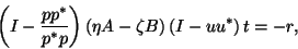 |
(226) |
with
 and
and
 .
It can be shown that if (8.13)
is solved exactly, the convergence to
the generalized eigenvalue will be quadratic;
see [408, Theorem 3.2].
Usually, this correction equation is solved
only approximately, for
instance, with a (preconditioned) iterative
solver. The obtained vector
.
It can be shown that if (8.13)
is solved exactly, the convergence to
the generalized eigenvalue will be quadratic;
see [408, Theorem 3.2].
Usually, this correction equation is solved
only approximately, for
instance, with a (preconditioned) iterative
solver. The obtained vector  is used for the expansion
  of and
 is used for the
expansion of . For both spaces we work with orthonormal bases.
Therefore, the new columns are orthonormalized with respect to the
current basis by a modified Gram-Schmidt orthogonalization process
(see §4.7.1).
is used for the
expansion of . For both spaces we work with orthonormal bases.
Therefore, the new columns are orthonormalized with respect to the
current basis by a modified Gram-Schmidt orthogonalization process
(see §4.7.1).
It can be shown that, with the above choices for  and ,
and ,
 |
(227) |
The relation between the partial generalized Schur
form for the given large problem and the
complete generalized Schur form for
the reduced problem (8.11) via
right vectors ( ) is
similar to the relation via left vectors
(
) is
similar to the relation via left vectors
( ). This can also
be exploited for restarts.
). This can also
be exploited for restarts.
Next: Deflation and Restart
Up: Jacobi-Davidson Method G. Sleijpen and
Previous: Jacobi-Davidson Method G. Sleijpen and
Contents
Index
Susan Blackford
2000-11-20