The Jacobi-Davidson method is based on a combination of two basic
principles. The first one is to apply a Galerkin approach for the
eigenproblem
![]() , with respect to some given subspace
spanned by an orthonormal basis
, with respect to some given subspace
spanned by an orthonormal basis
![]() . The usage of other
than Krylov subspaces was suggested by Davidson [99], who also
suggested specific choices,
different from the ones that we will take,
for the construction of orthonormal basis vectors
. The usage of other
than Krylov subspaces was suggested by Davidson [99], who also
suggested specific choices,
different from the ones that we will take,
for the construction of orthonormal basis vectors ![]() . The
Galerkin condition is
. The
Galerkin condition is
At this point the other principle behind the Jacobi-Davidson approach
comes into play. The idea goes back to Jacobi [241]. Suppose
that we have an eigenvector approximation ![]() for an
eigenvector
for an
eigenvector ![]() corresponding to a given eigenvalue
corresponding to a given eigenvalue ![]() . Then
Jacobi suggested (in the original paper for strongly diagonally dominant
matrices) computing the orthogonal correction
. Then
Jacobi suggested (in the original paper for strongly diagonally dominant
matrices) computing the orthogonal correction ![]() for
for ![]() so
that
so
that
From (4.48) we conclude that
![]() ,
and in particular that
,
and in particular that
![]() , so that the
Jacobi-Davidson correction equation represents a consistent linear system.
, so that the
Jacobi-Davidson correction equation represents a consistent linear system.
It can be shown that the exact solution of (4.49) leads to
cubic convergence of the largest
![]() towards
towards
![]() for increasing
for increasing ![]() (similar statements can be made
for the convergence towards other eigenvalues of
(similar statements can be made
for the convergence towards other eigenvalues of ![]() , provided that the
Ritz values are selected appropriately in each step).
, provided that the
Ritz values are selected appropriately in each step).
In [411] it is suggested to solve equation (4.49)
only approximately, for instance, by some steps of minimal residual (MINRES) [350],
with an appropriate preconditioner ![]() for
for
![]() , if
available, but in fact any approximation technique for
, if
available, but in fact any approximation technique for ![]() is
formally allowed, provided that the projectors
is
formally allowed, provided that the projectors
![]() are taken into account. In our
templates we will present ways to approximate
are taken into account. In our
templates we will present ways to approximate ![]() with Krylov
subspace methods.
with Krylov
subspace methods.
We will now discuss how to use preconditioning for an iterative solver
like generalized minimal residual (GMRES) or conjugate gradient squared (CGS),
applied to equation (4.49). Suppose that
we have a left preconditioner ![]() available for the operator
available for the operator
![]() , for which in some sense
, for which in some sense
![]() . Since
. Since
![]() varies with the
iteration count
varies with the
iteration count ![]() , so may the preconditioner, although it is often
practical to work with the same
, so may the preconditioner, although it is often
practical to work with the same ![]() for different values of
for different values of ![]() . Of
course, the preconditioner
. Of
course, the preconditioner ![]() has to be restricted to the subspace
orthogonal to
has to be restricted to the subspace
orthogonal to ![]() as well, which means that we have to work
with, efficiently,
as well, which means that we have to work
with, efficiently,
We assume that we use a Krylov solver with initial
guess ![]() and with left preconditioning for the approximate
solution of the correction equation (4.49). Since the
starting vector is in the subspace orthogonal to
and with left preconditioning for the approximate
solution of the correction equation (4.49). Since the
starting vector is in the subspace orthogonal to ![]() , all
iteration vectors for the Krylov solver will be in that space. In that
subspace we have to compute the vector
, all
iteration vectors for the Krylov solver will be in that space. In that
subspace we have to compute the vector
![]() for a vector
for a vector ![]() supplied by the
Krylov solver, and
supplied by the
Krylov solver, and
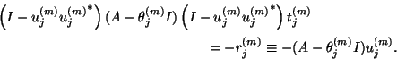
Since
![]() , it follows that
, it follows that ![]() satisfies
satisfies
![]() or
or
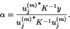
![]() . The condition
. The condition
![]() leads to
leads to
If we form an approximation for ![]() in (4.49) as
in (4.49) as
![]() , with
, with
![]() such that
such that
![]() and without
acceleration by an iterative solver, we obtain a process which was
suggested by Olsen, Jørgensen, and Simons [344].
and without
acceleration by an iterative solver, we obtain a process which was
suggested by Olsen, Jørgensen, and Simons [344].