An Algorithm Template.

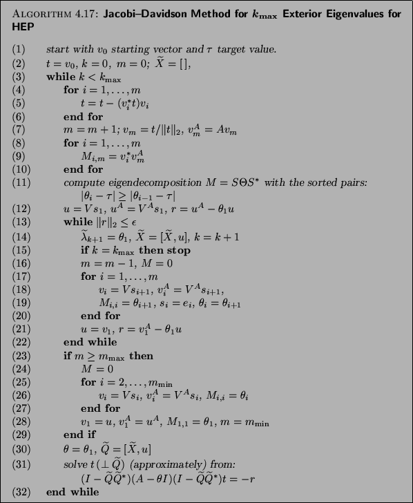
The complete algorithm for the Jacobi-Davidson method that includes restart with a number of Ritz vectors and deflation for the computation of a number of eigenpairs is called JDQR [172], since it can be interpreted as an iterative approach for the QR algorithm. The template for this algorithm is given in Algorithm 4.17.

To apply this algorithm we need to specify a starting vector ${v}_0$, a tolerance $\epsilon$, a target value $\tau$, and a number ${k}_{\max}$ that specifies how many eigenpairs near $\tau$ should be computed. The value of ${m}_{\max}$ denotes the maximum dimension of the search subspace. If it is exceeded, a restart takes place with a subspace of specified dimension ${m}_{\min}$.

On completion typically the ${k}_{\max}$ largest eigenvalues are delivered when $\tau$ is chosen larger than $\lambda_{\max}(A)$; the ${k}_{\max}$ smallest eigenvalues are delivered if $\tau$ is chosen smaller than $\lambda_{\min}(A)$. The computed eigenpairs $(\widetilde\lambda_j, \widetilde{x}_{j})$, $\Vert\widetilde{x}_{j}\Vert _2=1$, satisfy $\Vert A \widetilde{x}_{j}-\widetilde\lambda_j \widetilde{x}_{j}\Vert _2\leq j\epsilon$, where $\widetilde{x}_j$ denotes the $j$th column of $\widetilde{X}$.

In principle, this algorithm computes the ${k}_{\max}$ eigenvalues closest to a specified target value $\tau$. This is only reliable if the ${k}_{\max}$ largest or ${k}_{\max}$ smallest eigenvalues are wanted. For interior sets of eigenvalues we will describe safer techniques in §4.7.4. We will now comment on some parts of the algorithm in view of our discussions in previous subsections.

(2)

Initialization phase. The search subspace is initialized with $t=v_0$.

(4)-(6)

The new expansion vector for the search subspace is made orthogonal with respect to the current search subspace by means of modified Gram-Schmidt. This can be replaced, for improved numerical stability, by the template given in Algorithm 4.14.

If ${m}=0$, this is an empty loop.

(8)-(10)

We compute only the upper triangular part of the Hermitian matrix ${M}\equiv V^\ast AV$ (of order ${m}$).

(11)

The eigenproblem for the ${m}$ by ${m}$ matrix ${M}$ can be solved by a standard eigensolver for dense Hermitian eigenproblems from LAPACK. We have chosen to compute the standard Ritz values, which makes the algorithm suitable for computing the largest or smallest ${k}_{\max}$ eigenvalues of $A$. If one wishes to compute ${k}_{\max}$ eigenvalues somewhere in the interior of the spectrum, the usage of harmonic Ritz values is advocated; see §4.7.4.

The matrix ${V}$ denotes the $n$ by ${m}$ matrix with columns ${v}_j$, ${V^A}\equiv AV$ likewise; $S$ is the $m$ by $m$ matrix with columns $s_j$, and $\Theta = \diag(\theta_1,\ldots,\theta_m)$.

(13)

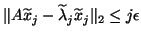
The stopping criterion is to accept an eigenvector approximation as soon as the norm of the residual (for the normalized eigenvector approximation) is below $\epsilon$. This means that we accept inaccuracies the order of $\epsilon^2$ in the computed eigenvalues and inaccuracies (in angle) in the eigenvectors in the order of $\epsilon$, provided that the associated eigenvalue is simple and well separated from the other eigenvalues; see (4.4).

Occasionally one of the wanted eigenvectors of $A$ may be undetected, for instance, if $v_0$ has no component in the corresponding eigenvector direction. For a random start vector this is rather unlikely. (See also note (14) for Algorithm 4.13.)

(16)

After acceptance of a Ritz pair, we continue the search for a next eigenpair, with the remaining Ritz vectors as a basis for the initial search space. These vectors are computed in (17)-(20).

(23)

We restart as soon as the dimension of the search space for the current eigenvector exceeds ${m}_{\max}$. The process is restarted with the subspace spanned by the ${m}_{\min}$ Ritz vectors corresponding to the Ritz values closest to the target value $\tau$ (and they are computed lines (25)-(27)).

(30)-(31)

We have collected the locked (computed) eigenvectors in $\widetilde{X}$, and the matrix $\widetilde{Q}$ is $\widetilde{X}$ expanded with the current eigenvector approximation ${u}$. This is done in order to obtain a more compact formulation; the correction equation is equivalent to the one in (4.50). The new correction ${t}$ has to be orthogonal to the columns of $\widetilde{X}$ as well as to ${u}$.

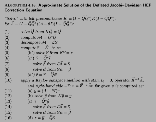
Of course, the correction equation can be approximately solved by any suitable process, for instance, by a preconditioned Krylov subspace method. Because of the occurrence of $\widetilde{Q}$ one has to be careful with the use of preconditioners for the matrix $A-\theta I$. The inclusion of preconditioners can be done following the same principles as for the single-vector Jacobi-Davidson algorithm; see Algorithm 4.18 for a template. Make sure that the starting vector ${t}_0$ for an iterative solver satisfies the orthogonality constraints $\widetilde{Q}^\ast {t}_0=0$. Note that significant savings per step can be made in Algorithm 4.18 if ${K}$ is kept the same for a (few) Jacobi-Davidson iterations. In that case columns of ${\widehat{Q}}$ can be saved from previous steps. Also the matrix ${\cal M}$ in Algorithm 4.18 can be updated from previous steps, as well as its ${\cal L}{\cal U}$ decomposition.