


Next: An Algorithm Template.
Up: Restart and Deflation
Previous: Deflation.
Contents
Index
Preconditioning for an iterative solver like GMRES or CGS, applied with
equation (4.50), is only slightly more complicated than in the
single-vector case (cf. §4.7.1). Suppose that we have a
left preconditioner  available for the operator
 . Let
. Let  denote the matrix
 expanded with
 as its
  th column. In this case, the preconditioner
has to be restricted to the subspace orthogonal to
as well, which means that we have to work effectively with
th column. In this case, the preconditioner
has to be restricted to the subspace orthogonal to
as well, which means that we have to work effectively with
Similar to the single-vector case, this can be realized in a surprisingly
efficient way.
Assume that we use a Krylov solver with initial guess  and with
left-preconditioning for the approximate solution of the correction
equation (4.50). Since the starting vector is in the subspace
orthogonal to , all iteration vectors for the Krylov
solver will be in that space. In that subspace we have to compute the
vector
and with
left-preconditioning for the approximate solution of the correction
equation (4.50). Since the starting vector is in the subspace
orthogonal to , all iteration vectors for the Krylov
solver will be in that space. In that subspace we have to compute the
vector
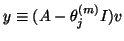
 for a vector
 supplied by the Krylov solver, and
This is done in two steps. First we compute
with
 since
since
 .
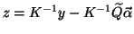
Then, with left-preconditioning we solve
.
Then, with left-preconditioning we solve
 from
from
Since
 , it follows that
  satisfies
 or
or
 .
The condition
leads to
.
The condition
leads to
The vector
 is solved from
 and, likewise,
 is solved from
 .
Note that the last set of equations has to be solved only once in an
iteration process for equation (4.50), so that effectively
.
Note that the last set of equations has to be solved only once in an
iteration process for equation (4.50), so that effectively
 operations with the preconditioner are required for
  iterations of the linear solver. Note also that a matrix-vector
multiplication with the left-preconditioned operator, in an iteration of
the Krylov solver, requires only one operation with
iterations of the linear solver. Note also that a matrix-vector
multiplication with the left-preconditioned operator, in an iteration of
the Krylov solver, requires only one operation with
 and
and
 , instead of the four actions of the
projector operator
, instead of the four actions of the
projector operator
 . This has been
worked out in the solution template, given in Algorithm 4.18.
Note that obvious savings can be realized if the operator is kept
the same for a number of successive eigenvalue computations (for
details, see [412]).
. This has been
worked out in the solution template, given in Algorithm 4.18.
Note that obvious savings can be realized if the operator is kept
the same for a number of successive eigenvalue computations (for
details, see [412]).
Next: An Algorithm Template.
Up: Restart and Deflation
Previous: Deflation.
Contents
Index
Susan Blackford
2000-11-20