Computing Interior Eigenvalues

If one is searching for the eigenpair with the smallest or largest eigenvalue only, then the obvious restart approach works quite well, but often it does not do very well if one is interested in an interior eigenvalue. The problem is that the Ritz values converge monotonically towards exterior eigenvalues, and a Ritz value that is close to a target value in the interior of the spectrum may be well on its way to some other exterior eigenvalue. It may even be the case that the corresponding Ritz vector has only a small component in the direction of the desired eigenvector. It will be clear that such a Ritz vector represents a poor candidate for restart and the question is, What is a better vector for restart? One answer is given by the so-called harmonic Ritz vectors, discussed in §3.2; see also [331,349,411].

As we have seen, the Jacobi-Davidson methods generate basis vectors ${v}_1, \ldots, {v}_{m}$ for a subspace ${\cal V}_{m}$. For the projection of $A$ onto this subspace we compute the vectors ${w}_j\equiv A{v}_j$. The harmonic Ritz values are inverses of the Ritz values of $A^{-1}$, with respect to the subspace spanned by the ${w}_j$. They can be computed without inverting $A$, since a harmonic Ritz pair $(\widetilde{\theta}_j^{(m)},\widetilde{u}_j^{(m)})$ satisfies

$$A\widetilde{u}_j^{(m)} - \widetilde{\theta}_j^{(m)} \widetil... ...\perp {\cal W}_{m} \equiv \mbox{span}({w}_1,\ldots , {w}_{m})$$ (60)

for $\widetilde{u}_j^{(m)} \in {V}_{m}$ and $\widetilde{u}_j^{(m)}\neq 0$. This implies that the harmonic Ritz values are the eigenvalues of the pencil $({W}_{m}^\ast A{V}_{m}, {W}_{m}^\ast {V}_{m})$, or, since ${W}_{m}=A{V}_{m}$:

$${W}_{m}^\ast {W}_{m} {s}_j^{(m)} - \widetilde{\theta}_j^{(m)} {W}_{m}^\ast {V}_{m} {s}_j^{(m)} =0 \, .\,$$

For stability reasons we orthonormalize the columns of ${W}_{m}$ and transform the columns of ${V}_{m}$ accordingly. This also further simplifies the equation: we see that the harmonic Ritz values are the inverses of the eigenvalues of the symmetric matrix ${W}_{m}^\ast {V}_{m}$.

In [349] it is shown that for Hermitian $A$ the harmonic Ritz values converge monotonically towards the smallest nonzero eigenvalues in absolute value. Note that the harmonic Ritz values are unable to identify a zero eigenvalue of $A$, since that would correspond to an infinite eigenvalue of $A^{-1}$. Likewise, the harmonic Ritz values for the shifted matrix $A-\tau I$ converge monotonically towards eigenvalues $\lambda\neq \tau$ closest to the target value $\tau$. Fortunately, the search subspace ${\cal V}_m$ for the shifted matrix and the unshifted matrix coincide, which facilitates the computation of harmonic Ritz pairs for any shift. The harmonic Ritz vector for the shifted matrix, corresponding to the harmonic Ritz value closest to $\tau$, can be interpreted as maximizing a Rayleigh quotient for $(A-\tau I)^{-1}$. It represents asymptotically the best information that is available for the wanted eigenvalue, and hence it represents asymptotically the best candidate as a starting vector after restart, provided that $\tau\neq \lambda$.

For harmonic Ritz values, the correction equation has to take into account the orthogonality with respect to $A\tilde u^{(m)}_j$, and this leads to skew projections. We can use orthogonal projections in the following way. If $\tilde u=\tilde u^{(m)}_j$ is the selected approximation of an eigenvector, the Rayleigh quotient $\theta = \tilde u^\ast A\tilde u/\tilde u^\ast \tilde u$ leads to the residual with smallest norm; that is, with $r\equiv A\tilde u-\theta \tilde u$, we have that $\Vert r\Vert _2\leq \Vert A\tilde u-\mu\tilde u\Vert _2$ for any scalar $\mu$, including the harmonic Ritz value $\mu=\tilde\theta^{(m)}_j$. Moreover, the residual $r$ for the Rayleigh quotient is orthogonal to $\tilde u$. This makes $r$ ``compatible'' with the operator $(I- u u^\ast)(A-\theta I)(I-u u^\ast)$ in the correction equation. Here $u\equiv \tilde u/\Vert\tilde u\Vert _2$.

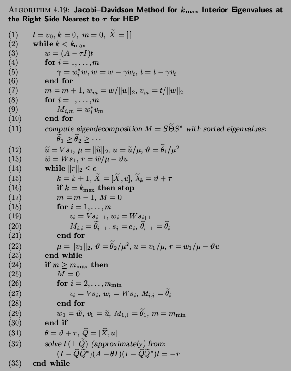
An algorithm for the Jacobi-Davidson method based on harmonic Ritz values and vectors, combined with restart and deflation, is given in Algorithm 4.19. The algorithm can be used for the computation of a number of successive eigenvalues immediately to the right of the target value $\tau$.

To apply this algorithm we need to specify a starting vector ${v}_0$, a tolerance $\epsilon$, a target value $\tau$, and a number ${k}_{\max}$ that specifies how many eigenpairs near $\tau$ should be computed. The value of ${m}_{\max}$ denotes the maximum dimension of the search subspace. If it is exceeded, a restart takes place with a subspace of specified dimension ${m}_{\min}$.

On completion, the ${k}_{\max}$ eigenvalues at the right side nearest to $\tau$ are delivered. The computed eigenpairs $(\widetilde\lambda_j, \widetilde{x}_{j})$, $\Vert\widetilde{x}_{j}\Vert _2=1$, satisfy $\Vert A \widetilde{x}_{j}-\widetilde\lambda_j \widetilde{x}_{j}\Vert _2\leq j\epsilon$, where $\widetilde{x}_j$ denotes the $j$th column of $\widetilde{X}$.

For exterior eigenvalues a simpler algorithm has been described in §4.7.3. We will now comment on some parts of the algorithm in view of our discussions in previous subsections.

(1)

Initialization phase.

(3)-(7)

The vector $w = (A-\tau I)t$ is made orthogonal with respect to the current test subspace ${\cal W}_{m}$ by means of modified Gram-Schmidt. This can be replaced, for improved numerical stability, by an adoption (for the vector $t$) of the template given in Algorithm 4.14.

(8)-(10)

The values ${M}_{i,j}$ represent elements of the square ${m}$ by ${m}$ matrix ${M}\equiv {W}^\ast {V}$, where ${V}$ denotes the $n$ by ${m}$ matrix with columns ${v}_j$, and likewise ${W}$. Because ${M}$ is Hermitian, only the upper triangular part of this matrix is computed.

(11)-(13)

At this point the eigenpairs for the problem ${M}{s}=\widetilde\theta {s}$ should be computed. This can be done with a suitable routine for Hermitian dense matrices from LAPACK. Note that the harmonic Ritz values are the inverses of the eigenvalues of ${M}$. We have to compute the Rayleigh quotient $\theta$ for ${V}{s}_1$, and next normalize ${V}{s}_1$, in order to compute a proper residual $r \perp {V}{s}_1$. We have used that ${s}_1^\ast {V}^\ast (A-\tau I) {V}{s}_1 = {s}_1^\ast {M}^\ast {s}_1=\widetilde\theta_1$.

The vectors $s_j$ are the columns of $m$ by $m$ matrix $S$ and $\tilde\Theta = \diag(\widetilde\theta_1,\ldots,\widetilde\theta_m)$.

(14)

The stopping criterion is to accept an eigenvector approximation as soon as the norm of the residual (for the normalized eigenvector approximation) is below $\epsilon$. This means that we accept inaccuracies in the order of $\epsilon^2$ in the computed eigenvalues, and inaccuracies (in angle) in the eigenvectors of ${\cal O}({\epsilon})$, provided that the associated eigenvalue is simple and well separated from the others; see (4.4).

Detection of all wanted eigenvalues cannot be guaranteed; see note (14) for Algorithm 4.13 and note (13) for Algorithm 4.17.

(17)

This is a restart after acceptance of an approximate eigenpair. The restart is slightly more complicated since two subspaces are involved. Recomputation of the spanning vectors from these subspaces is done in (18)-(21).

(24)

At this point we have a restart when the dimension of the subspace exceeds ${m}_{\max}$. After a restart, the Jacobi-Davidson iterations are resumed with a subspace of dimension ${m}_{\min}$. The selection of this subspace is based on the harmonic Ritz values nearest to the target $\tau$.

(31)-(32)

The deflation with computed eigenvectors is represented by the factors with $\widetilde{X}$. The matrix $\widetilde{X}$ has the computed eigenvectors as its columns. If a left preconditioner ${K}$ is available for the operator $A-\theta I$, then with a Krylov solver similar reductions are realizable, as in the situation for exterior eigenvalues. A template for the efficient handling of the left-preconditioned operator is given in Algorithm 4.18.