Algorithm.

In the direct iteration variant, we multiply with $A$ and solve systems with $B$; this corresponds to $C=B^{-1}A$. It computes a basis $V_j$, where the matrix pencil $\{A,B\}$ is represented by a real symmetric tridiagonal matrix,

$$T_{j}=\left[ \begin{array}{cccc}\alpha_1 & \beta_1 &&\\ \be... ...beta_{j-1}\\ &&\beta_{j-1}&\alpha_j\\ \end{array} \right]\;,$$ (72)

satisfying the basic recursion,

$$AV_j=BV_{j}T_{j}+re_j^{\ast}\;.$$ (73)

Compare this to the standard Hermitian case (4.10). Now the basis $V_j$ is $B$-orthogonal,

$$V_j^{\ast}BV_j=I_{j}\,,$$ (74)

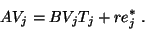
and the matrix $T$ is congruent to a section of $A$,

$$V_j^{\ast}AV_j=T_{j}\,.$$ (75)

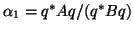
We simplify the description of the $B$-orthogonalization by introducing an auxiliary basis,

$$W_j=BV_j\,,$$ (76)

which is $B^{-1}$-orthogonal,

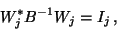$$W_j^{\ast}B^{-1}W_j=I_{j}\,,$$ (77)

and for which $W^{\ast}V=I$.

Precisely as in the standard case, compute an eigensolution of $T_{j}$,

$$T_{j}s_i^{(j)}=s_i^{(j)}\theta_i^{(j)},$$

and get a Ritz value $\theta_i^{(j)}$ and a Ritz vector,

$$x_i^{(j)}=V_js_i^{(j)},$$ (78)

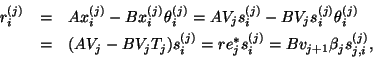
approximating an eigenpair of the pencil (5.1). Its residual,

$$\begin{eqnarray*} r_i^{(j)}& = & Ax_i^{(j)}-Bx_i^{(j)}\theta_i^{(j)} =AV_js_i^{(... ...j})s_i^{(j)} =re_j^{\ast}s_i^{(j)}=Bv_{j+1}\beta_js_{j,i}^{(j)}, \end{eqnarray*}$$

is $B$-orthogonal to the Krylov space spanned by $V_j$.

We may estimate the norm of the residual as we did in the standard Hermitian case, (4.13), but now this is better done using the $B^{-1}$-norm getting

$$\Vert r_i^{(j)}\Vert _{B^{-1}}=\vert\beta_js_{j,i}^{(j)}\vert\;,$$ (79)

using the fact that $(Bv_{j+1})^{\ast}B^{-1}(Bv_{j+1})=v_{j+1}^{\ast}Bv_{j+1}$. It is natural to use the $B^{-1}$-norm when measuring convergence; see [353, Chap. 15].

As in the standard case we need to monitor the subdiagonal elements $\beta_j$ of $T$, and the last elements $s_{j,i}^{(j)}$ of its eigenvectors. As soon as this product is small, we may flag an eigenvalue as converged, without actually performing the matrix-vector multiplication (5.14). We save this operation until the step $j$ when the estimate (5.15) indicates convergence.

We get the following algorithm.

Let us comment on this algorithm step by step:

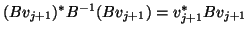
(1)

If a good guess for the wanted eigenvector is available, use it as the starting $q$. In other cases choose a random direction, for instance, one consisting of normally distributed random numbers. Notice that $\alpha_1=q^{\ast}Aq/(q^{\ast}Bq)$ is the Rayleigh quotient of the starting vector and that $\beta_1$ measures the $B^{-1}$-norm of its residual (5.15).

(4)

This is where the large matrix $A$ comes in. Any routine that performs a matrix-vector multiplication can be used.

(8)

It is sufficient to reorthogonalize just one of the bases $V$ or $W$, not both of them. The choices are the same as in the standard case:

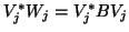
1. Full: Now we want to make the $v$ basis vectors $B$-orthogonal, computing
   
   $$r=r-B(V_j(V_j^{\ast}r))$$
   
   
   and repeat until the vector $r$ is orthogonal to the basis $V_j$. We have to apply one matrix-vector multiplication by $B$ for each reorthogonalization, and we have to use the classical variant of the Gram-Schmidt process.

   We may avoid these extra multiplications with $B$ if we save both bases $V_j$ and $W_j$ and subtract multiples of the columns of $W_j$,
   

   $$r=r-W_j(V_j^{\ast}r)\,,$$
   
   
   until orthogonality is obtained, almost always just once. Now we may use a modified Gram-Schmidt orthogonalization.

2. Selective: Reorthogonalize only when necessary, one has to monitor the orthogonality as described in §4.4.4 for the standard case. Note that now the symmetric matrix $V_j^{\ast}W_j=V_j^{\ast}BV_j$ is involved and some of the vectors $v_k$ have to be replaced by the corresponding vectors $w_k$.
3. Local: Used for huge matrices, when it is difficult to store the whole basis $V_j$. Advisable only when one or two extreme eigenvalues are sought. We make sure that $w_{j+1}$ is orthogonal to $v_{j-1}$ and $v_j$ by subtracting $r=r-w_{j-1}(v_{j-1}^{\ast}r); r=r-w_j(v_j^{\ast}r)\,$ once in this step.

(9)

Here we need to solve a system with the positive definite matrix $B$. This was not needed in the standard case (4.1).

(11)

For each step $j$, or at appropriate intervals, compute the eigenvalues $\theta_i^{(j)}$ and eigenvectors $s_i^{(j)}$ of the symmetric tridiagonal matrix $T_{j}$ (5.8). Same procedure as for the standard case.

(12)

The algorithm is stopped when a sufficiently large basis $V_j$ has been found, so that eigenvalues $\theta_i^{(j)}$ of the tridiagonal matrix $T_{j}$ (5.8) give good approximations to all the eigenvalues of the pencil (5.1) sought.

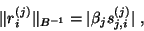
The estimate (5.15) for the residual may be too optimistic if the basis $V_j$ is not fully $B$-orthogonal. Then the Ritz vector $x_i^{(j)}$ (5.14) may have its norm smaller than $1$, and we have to replace the estimate by,

$$\Vert r_i^{(j)}\Vert=\vert\beta_js_{j,i}^{(j)}\vert/\Vert V_js_i^{(j)}\Vert _B\;.$$

(14)

The eigenvectors of the original matrix pencil (5.1) are computed only when the test in step (5.4) has indicated that they have converged. Then the basis $V_j$ is used in a matrix-vector multiplication to get the eigenvector (5.14),

$$x_i^{(j)}=V_js_i^{(j)},$$

for each $i$ that is flagged as converged.