Lanczos Method
  A. Ruhe

The Lanczos algorithm is closely related to the iterative algorithms discussed in the previous section in that it needs to access the matrix only in the form of matrix-vector operations. It is different in that it makes much better use of the information obtained by remembering all the directions computed and always lets the matrix operate on a vector orthogonal to all those previously tried.

In this section we describe the Hermitian Lanczos algorithm applicable to the eigenvalue problem,

$$Ax=\lambda x\;,$$ (20)

where $A$ is a Hermitian, or in the real case symmetric, matrix operator.

The algorithm starts with a properly chosen starting vector $v$ and builds up an orthogonal basis $V_j$ of the Krylov subspace,

$${\cal K}^j(A,v)=\mbox{span}\{v,VA,A^2v,\dots,A^{j-1}v\}\;,$$ (21)

one column at a time. In each step just one matrix-vector multiplication

$$y=Ax$$ (22)

is needed. In the new orthogonal basis $V_j$ the operator $A$ is represented by a real symmetric tridiagonal matrix,

$$T_{j}=\left[ \begin{array}{cccc}\alpha_1 & \beta_1 &&\\ \be... ...beta_{j-1}\\ &&\beta_{j-1}&\alpha_j\\ \end{array} \right]\;,$$ (23)

which is also built up one row and column at a time, using the basic recursion,

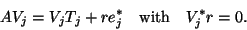$$AV_j=V_{j}T_{j}+re_j^{\ast} \quad \mbox{with} \quad V^{\ast}_j r = 0.$$ (24)

At any step $j$, we may compute an eigensolution of $T_{j}$,

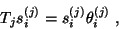$$T_{j}s_i^{(j)}=s_i^{(j)}\theta_i^{(j)}\;,$$ (25)

where the superscript $(j)$ is used to indicate that these quantities change for each iteration $j$. The Ritz value $\theta_i^{(j)}$ and its Ritz vector,

$$x_i^{(j)}=V_js_i^{(j)}\;,$$ (26)

will be a good approximation to an eigenpair of $A$ if the residual has small norm; see §4.8.

Let us compute the residual for this Ritz pair,

$$r_i^{(j)}=Ax_i^{(j)}-x_i^{(j)}\theta_i^{(j)} =AV_js_i^{(j)}-V... ...^{(j)}=(AV_j-V_jT_{j})s_i^{(j)}= v_{j+1}\beta_js_{j,i}^{(j)}\;.$$

We see that its norm satisfies

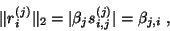$$\Vert r_i^{(j)}\Vert _2=\vert\beta_js_{i,j}^{(j)}\vert=\beta_{j,i}\;,$$ (27)

so we need to monitor only the subdiagonal elements $\beta_j$ of $T$ and the last elements $s_{i,j}^{(j)}$ of its eigenvectors to get an estimate of the norm of the residual. As soon as this estimate is small, we may flag the Ritz value $\theta_i^{(j)}$ as converged to the eigenvalue $\lambda_i$. Note that the computation of the Ritz values does not need the matrix-vector multiplication (4.12). We can save this time-consuming operation until the step $j$, when the estimate () indicates convergence.