


Next: Convergence Properties
Up: Lanczos Method A.
Previous: Lanczos Method A.
Contents
Index
We get the following algorithm.
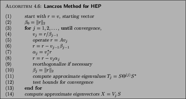
Let us comment on some of the steps of Algorithm 4.6:
- (1)
- If a good guess
for the wanted eigenvector is available, use it. For instance, if,
for a discretized partial differential equation,
it is known that the wanted eigenvector
is smooth with respect to the grid, one could start with a vector
with all ones. In other cases
choose a random direction, for instance, one consisting of normally
distributed random numbers.
- (5)
- This matrix-vector operation is most often the CPU-dominating
work. Any routine that performs a matrix-vector multiplication can
be used. In the shift-and-invert case, solve systems with the
factored matrix. There is, as of now, little solid experience of
using iterative equation solvers in the inverted case.
- (9)
- When computing in finite precision,
orthogonality is lost as soon as one eigenvalue converges.
The choices for reorthogonalization are:
- Full:
Simple to implement; see §4.4.4 below. Iterations will
need successively more work as
 increases. This is the preferred choice in
the shift-and-invert case, when several eigenvalues converge in few
steps .
increases. This is the preferred choice in
the shift-and-invert case, when several eigenvalues converge in few
steps .
- Selective:
The most elaborate scheme, necessary when
convergence is slow and several eigenvalues are sought.
This option is also discussed later in §4.4.4.
- Local:
Used for huge matrices, when it is difficult to
store the whole basis
 . We make sure that
  is orthogonal to
 and
and  by doing an extra orthogonalization against
these two vectors, subtracting
by doing an extra orthogonalization against
these two vectors, subtracting
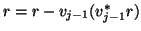 and
and
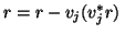 once in this step. Still we need to
detect and discard spurious eigenvalue approximations using
the Cullum device; see §4.4.4.
once in this step. Still we need to
detect and discard spurious eigenvalue approximations using
the Cullum device; see §4.4.4.
- (11)
- For each step , or at appropriate intervals, compute the
eigenvalues
 and eigenvectors
  of the
tridiagonal matrix
of the
tridiagonal matrix  (4.9).
If fast convergence is expected, as for shift-and-invert
problems, will be much smaller than  ; then this computation
is very fast and standard software from, e.g., LAPACK [12] is
recommended.
; then this computation
is very fast and standard software from, e.g., LAPACK [12] is
recommended.
If the Lanczos algorithm is applied directly to  and a large tridiagonal matrix
is computed, there are special tridiagonal eigenvalue algorithms
based on bisection and a Givens recursion for eigenvectors;
see [356,358,128] and §4.2.
and a large tridiagonal matrix
is computed, there are special tridiagonal eigenvalue algorithms
based on bisection and a Givens recursion for eigenvectors;
see [356,358,128] and §4.2.
- (12)
- The algorithm is
stopped when a sufficiently large basis has been found, so
that eigenvalues
of the tridiagonal matrix
(4.9) give good approximations to all the
eigenvalues of sought.
The estimate  (4.13)
for the residual may be too
optimistic if the basis is not fully orthogonal. Then the
Ritz vector
(4.13)
for the residual may be too
optimistic if the basis is not fully orthogonal. Then the
Ritz vector  (4.12) may have a norm
smaller than
(4.12) may have a norm
smaller than  , and we have to replace the estimate (
![[*]](http://www.netlib.org/utk/icons/crossref.png) ) by
) by
- (14)
- The eigenvectors of the original matrix are computed only when the
test in step (12) has indicated that they have
converged. Then the basis is used in a matrix-vector
multiplication to get the eigenvector (4.12),
for each  that is flagged as having converged.
The great beauty of this type of algorithm is that the matrix is
accessed only in a matrix-vector operation in step (5) in
Algorithm 4.6. Any type of sparsity and any
storage scheme can be taken advantage of.
It is necessary to keep only three vectors,  , , and ,
readily accessible; older vectors can be left on backing storage.
There is even a variant where only two vectors are needed
(see [353, Chap. 13.1]), but it demands some dexterity
to code it.
Except for the matrix-vector multiplication,
only scalar products and additions of
a multiple of a vector to another are needed. We recommend using
Level 1 BLAS routines; see §10.2.
, , and ,
readily accessible; older vectors can be left on backing storage.
There is even a variant where only two vectors are needed
(see [353, Chap. 13.1]), but it demands some dexterity
to code it.
Except for the matrix-vector multiplication,
only scalar products and additions of
a multiple of a vector to another are needed. We recommend using
Level 1 BLAS routines; see §10.2.
Next: Convergence Properties
Up: Lanczos Method A.
Previous: Lanczos Method A.
Contents
Index
Susan Blackford
2000-11-20