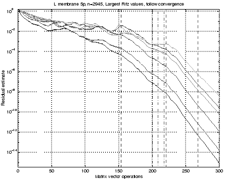
We have plotted the estimated residuals (4.13) for
the six largest eigenvalues as a function of the number ![]() of Lanczos
steps in Figure 4.1. The curves show the residual
estimates (4.13) for each step and were computed only
for illustration purposes after the actual computation. The LANSO
algorithm called the QL algorithm to compute eigenvalues and last
elements of eigenvectors to test for convergence
(4.13),
at the iterations
marked with dashdotted vertical
lines in the plot. The selective orthogonalization triggered
reorthogonalization at the steps we marked with dashed lines,
altogether only three times during all these
of Lanczos
steps in Figure 4.1. The curves show the residual
estimates (4.13) for each step and were computed only
for illustration purposes after the actual computation. The LANSO
algorithm called the QL algorithm to compute eigenvalues and last
elements of eigenvectors to test for convergence
(4.13),
at the iterations
marked with dashdotted vertical
lines in the plot. The selective orthogonalization triggered
reorthogonalization at the steps we marked with dashed lines,
altogether only three times during all these ![]() steps. This is typical
for situations with a slow convergence: orthogonality is preserved
until the first Ritz value converges.
steps. This is typical
for situations with a slow convergence: orthogonality is preserved
until the first Ritz value converges.
Note that a relatively large number of steps, about ![]() , are needed to bring the
residual of the leading eigenvalue down to
, are needed to bring the
residual of the leading eigenvalue down to ![]() , and that another
, and that another
![]() steps are taken before full machine accuracy is reached.
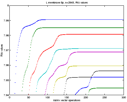
Looking at the Ritz values
steps are taken before full machine accuracy is reached.
Looking at the Ritz values
![]() of (4.11) plotted
versus
of (4.11) plotted
versus ![]() in Figure 4.2, we see that the largest Ritz value grows
with
in Figure 4.2, we see that the largest Ritz value grows
with ![]() until around step
until around step ![]() , when it stabilizes. Frequently a
Ritz value will start to approach one eigenvalue, but will later move to
another, not yet found, eigenvalue. This happens with the third Ritz
value at steps
, when it stabilizes. Frequently a
Ritz value will start to approach one eigenvalue, but will later move to
another, not yet found, eigenvalue. This happens with the third Ritz
value at steps ![]() to
to ![]() and becomes more pronounced with the sixth
between steps
and becomes more pronounced with the sixth
between steps ![]() and
and ![]() . This phenomenon shows up in a less
evident fashion in Figure 4.1, where the third and sixth
curves from the bottom have plateaus at the steps when a Ritz value
shifts allegiance. A user of a direct Lanczos method is advised to take care
when deciding whether all the largest eigenvalues really have
converged.
. This phenomenon shows up in a less
evident fashion in Figure 4.1, where the third and sixth
curves from the bottom have plateaus at the steps when a Ritz value
shifts allegiance. A user of a direct Lanczos method is advised to take care
when deciding whether all the largest eigenvalues really have
converged.