


In [Fox:86a;92c;92h;93a], we point out some interesting features of the physical analogy and energy function introduced in Section 11.1.4.
Suppose that we are using the simulating annealing method of
Section 11.1.4 on a dynamically varying system. Assume that
this annealing algorithm is running in parallel in the same machine on
which the problem executes. Suppose that we use a (reasonably)
optimal annealing strategy. Even in this case, the ``heatbath''
formed by load balancer and operating system can
only ``cool'' the problem to a minimum temperature  . At this
temperature, any further gains from improved decomposition by lowering
the temperature will be outweighed by time taken to perform the
annealing. This temperature
. At this
temperature, any further gains from improved decomposition by lowering
the temperature will be outweighed by time taken to perform the
annealing. This temperature  is independent of
performance of computer; it is a property of the system being
simulated. Thus, we can consider this temperature
is independent of
performance of computer; it is a property of the system being
simulated. Thus, we can consider this temperature  as a new
property of a dynamical complex system. High
values of
as a new
property of a dynamical complex system. High
values of  imply that the system is rapidly varying; low values
that it is slowly varying.
imply that the system is rapidly varying; low values
that it is slowly varying.
Now we want to show that decompositions can lead to phase
transitions between different states of the
physical system defined by analogy of Section 11.1.2. In
the language of Chapter 3, we can say that the complex
system representing this problem exhibits a phase transition. We
illustrate this with a trivial particle dynamics problem shown in Figure 11.19. Typically, we use on
such problems the domain decomposition of Figure 11.19(a),
where each node of the parallel machine contains a single connected
region (compare Section 12.4). Alternatively, we can use the
scattered decomposition-described for
matrices in Section 8.1 and illustrated in
Figure 11.19(b). One assigns to each processor several small
regions of the space scattered uniformly throughout the domain. Each
processor gets ``a piece of the action'' and shares those parts of the
domain where the particle density and hence computational work is
either large or small. This was explored for partial differential
equations in [Morison:86a]. The scattered decomposition is a
local minimum-there is an optimal size for the scattered blocks of
space assigned to each processor. Both in this example and generally,
the scattered decomposition is not as good as domain decomposition.
This is shown in Figure 11.19(c), which sketches the energy
H as a function of the chosen decomposition. Now, suppose that the
particles move in time from t to  as shown in
Figure 11.19(d). The scattered decomposition minimum is unchanged, but as shown in Figure 11.19(c),(d) the domain
decomposition minimum moves with time.
as shown in
Figure 11.19(d). The scattered decomposition minimum is unchanged, but as shown in Figure 11.19(c),(d) the domain
decomposition minimum moves with time.
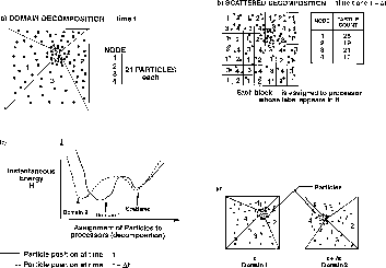
Figure 11.19: Particle Dynamics Problem on a Four-node System with Two
Decompositions (a) Domain, Time t, (b) Scattered Times t and
 , (c) Instantaneous Energies, (d) Domain Decomposition
Changing from Time t to
, (c) Instantaneous Energies, (d) Domain Decomposition
Changing from Time t to 
Now, one would often be interested not in the instantaneous energy H, but rather in the average
For this new objective function  , the scattered
decomposition can be the global minimum as illustrated in
Figure 11.20. The domain decomposition is smeared with time
and so its minimum is raised in value; the value of H at the
scattered decomposition minimum is unchanged. We can study
, the scattered
decomposition can be the global minimum as illustrated in
Figure 11.20. The domain decomposition is smeared with time
and so its minimum is raised in value; the value of H at the
scattered decomposition minimum is unchanged. We can study  as a function of
  , and the hardware ratio
  used in Equation 3.10. As
  increases or
  decreases, we move from the situation of
Figure 11.19(c) to that of Figure 11.20. In
physics language,
decreases, we move from the situation of
Figure 11.19(c) to that of Figure 11.20. In
physics language,  and
and  are order parameters which
control the phase transition between the two states scattered and
domain. Rapidly varying systems (high
are order parameters which
control the phase transition between the two states scattered and
domain. Rapidly varying systems (high  ), rather than those with
lower
), rather than those with
lower  , are more likely to see the transition as
  increases.
This agrees with physical intuition, as we now describe. When
increases.
This agrees with physical intuition, as we now describe. When  is
small (slowly varying system), domain decomposition is the global
minimum and this switches to a scattered decomposition as
is
small (slowly varying system), domain decomposition is the global
minimum and this switches to a scattered decomposition as  increases. In Figure 11.19(a),(b), we can associate with each
particle in the simulation a spin value which indicates the label of
the processor to which it is assigned. Then we see the direct analogy
to physical spin systems. At high temperatures, we have spin waves
(scattered decomposition); at low temperatures, (magnetic) domains
(domain decomposition).
increases. In Figure 11.19(a),(b), we can associate with each
particle in the simulation a spin value which indicates the label of
the processor to which it is assigned. Then we see the direct analogy
to physical spin systems. At high temperatures, we have spin waves
(scattered decomposition); at low temperatures, (magnetic) domains
(domain decomposition).
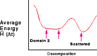
Figure: The Average Energy  of Equation 11.13
We end by noting that in the analogy there is a class of problems which we call microscopically dynamic. These are explored in [Fox:88f], [Fox:88kk;88uu]. In this problem class, the fundamental entities (particles in above analogy) move between nodes of parallel machine on a microscopic time scale. The previous discussion had only considered the adiabatic loosely synchronous problems where one can assume that the data elements (particles in the analogy) can be treated as fixed in a particular processor at each time instant. We will not give a general discussion here, but rather just illustrate the ideas with one example-the global sum calculation written in Fortran as
DO l I=l, LIMIT1
A(I)=0
DO 1 J=l, LIMIT2
1 A(I)=A(I) + B(I,J)
This is illustrated in Figure 11.21 (Color Plate) for the case LIMIT1=4 decomposed onto a four-node machine. The value of LIMIT1 is important for performance considerations but irrelevant for the discussion here. The optimal scheduling of communication and calculation is tricky and is discussed as the fold algorithm in [Fox:88a]. The four tasks of calculating the four A(I) cannot be viewed as particles as they move from node to node and we cannot represent this movement in the formalism used up to now. Rather, we now represent the tasks by ``space-time'' strings or world lines and one replaces Equation 11.9 by a Hamiltonian which describes interacting strings rather than interacting particles. This can be applied to event-driven simulations, message routing, and other microscopically dynamic problems. The strings need to be draped over the space-time grid formed by the complex computer as it evolves in time. Figure 11.21 (Color Plate) shows this compact ``draping'' for the fold algorithm.
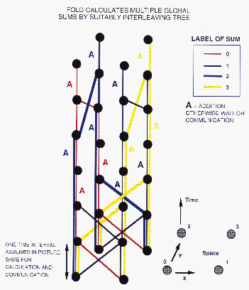
Figure 11.21: The Fold Algorithm. Four global sums
interleaved optimally on four processors.
We have successfully applied similar ideas to multivehicle and multiarm robot path planning and routing problems [Chiu:88f], [Fox:90e;90k;92c], [Gandhi:90a]. Comparison of the vehicle navigation in Figure 11.22 (Color Plate) with the computational routing problem in Figure 11.21 (Color Plate) illustrates the analogy.
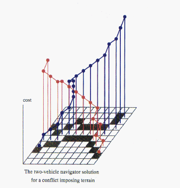
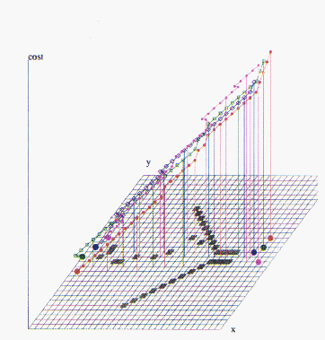
Figure 11.22: Two- and four-vechcle navigation
problems. in each case, vehicles have been given initial and final target
positions. The black squares are impassable and define a narrow pass.
Physical optimisation methods[Fox:88ii;90e] were used to find solutions.
