11.1.4 Simulated Annealing

Simulated annealing [Fox:88mm], [Hajek:88a], [Kirkpatrick:83a], [Otten:89a] is a very general optimization method which stochastically simulates the slow cooling of a physical system. The idea is that there is a cost function H (in physical terms, a Hamiltonian) which associates a cost with a state of the system, a ``temperature'' T, and various ways to change the state of the system. The algorithm works by iteratively proposing changes and either accepting or rejecting each change. Having proposed a change we may evaluate the change in H. The proposed change may be accepted or rejected by the Metropolis  criterion; if the cost function decreases the change is accepted unconditionally; otherwise it is accepted but only with probability . A crucial requirement for the proposed changes is reachability or ergodicity-that there be a sufficient variety of possible changes that one can always find a sequence of changes so that any system state may be reached from any other.

When the temperature is zero, changes are accepted only if H decreases, an algorithm also known as hill-climbing, or more generally, the greedy algorithm  [Aho:83a]. The system soon reaches a state in which none of the proposed changes can decrease the cost function, but this is usually a poor optimum. In real life, we might be trying to achieve the highest point of a mountain range by simply walking upwards; we soon arrive at the peak of a small foothill and can go no further.

On the contrary, if the temperature is very large, all changes are accepted, and we simply move at random ignoring the cost function. Because of the reachability property of the set of changes, we explore all states of the system, including the global optimum.

Simulated annealing consists of running the accept/reject algorithm between the temperature extremes. We propose many changes, starting at a high temperature and exploring the state space, and gradually decreasing the temperature to zero while hopefully settling on the global optimum. It can be shown that if the temperature decreases sufficiently slowly (the inverse of the logarithm of the time), then the probability of being in a global optimum tends to certainty [Hajek:88a].

Figure 11.4 shows simulated annealing applied to the load-balancing cost function in one dimension. The graph to be colored is a periodically connected linear array of 200 nodes, to be colored with four colors. The initial configuration, at the bottom of the figure, is the left 100 nodes colored white, two domains of 50 each in mid grays, and with no nodes colored in the darkest gray. We know that the global optimum is 50 nodes of each color, with all the nodes of the same color consecutive. Iterations run up the figure with the final configurations at the top.

  
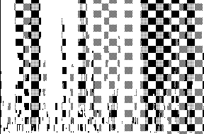
Figure 11.4: Simulated Annealing of a Ring Graph of Size 200, with the Four Graph Colors Shown by Gray Shades. The time history of the annealing runs vertically, with the maximum temperature and the starting configuration at the bottom, and zero temperature and the final optimum at the top. The basic move is to change the color of a graph node to a random color.

At each iteration of the annealing, a random node is chosen, and its color changed to a random color. This proposed move is accepted if the Metropolis criterion is accepted. At the end of the annealing, a good balance is achieved at the top of the figure, with each color having equal numbers of nodes; but there are 14 places where the color changes (communication cost = 14), rather than the minimum four.

Heuristics 

In choosing the change to be made to the state of the system, there may be intuitive or heuristic reasons to choose a change which tends to reduce the cost function. For our example of load balancing, we know that the optimal coloring of the graph has equal-sized compact ``globules''; if we were to restrict the new color of a node to the color of one of its two neighbors, then the boundaries between colors move without creating new domains.

The effect of this algorithm is shown in Figure 11.5, with the same number of iterations as Figure 11.4. The imbalance of 100 white nodes is quickly removed, but there are only three colors of 67 nodes each in the (periodically connected) final configuration. The problem is that the changes do not satisfy reachability; if a color is not present in graph coloring, then it can never come back.

  
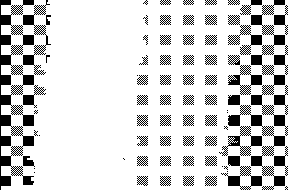
Figure: Same as Figure 11.4, Except the Basic Move Is to Change the Color of a Graph Node to the Color of One of the Neighbors.

Even if reachability is satisfied, a heuristic may degrade the quality of the final optimum, because a heuristic is coercing the state toward local minima in much the same way that a low temperature would. This may reduce the ability of the annealing algorithm to explore the state space, and cause it to drop into a local minimum and stay there, resulting in poor performance overall.

Figure 11.6 shows a solution to this problem. There is a high probability the new color is one of the neighbors, but also a small probability of a ``seed'' color, which is a randomly chosen color. Now we see a much better final configuration, close to the global optimum. The balance is perfect and there are five separate domains instead of the optimal four.

  
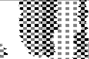
Figure: Same as Figure 11.4, Except the Basic Move Is to Change the Color of a Graph Node to the Color of One of the Neighbors with Large Probability, and to a Random Color with Small Probability.

Collisional Simulated Annealing

As presented so far, simulated annealing is a sequential algorithm, since whenever a move is made an acceptance decision must be made before another move may be evaluated. A parallel variant, which we shall call collisional simulated annealing,  would be to propose several changes to the state of the system, evaluate the Metropolis criterion on each simultaneously, then make those changes which are accepted. Figure 11.7 shows the results of the same set of changes as Figure 11.6, but doing 16 changes simultaneously instead of sequentially. Now there are eight domains in the final configuration rather than five. The essential difference from the sequential algorithm is that resulting from several simultaneous changes is not the sum of the values if the changes are made in sequence. We tend to get parallel collisions,  where there may be two changes, each of which is beneficial, but which together are detrimental. For example, a married couple might need to buy a lawnmower;  if either buys it, the result is beneficial to the couple, but if both simultaneously buy lawn mowers, the result is detrimental because they only need one.

  
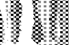
Figure: Same as Figure 11.6, Except the Optimization Is Being Carried Out in Parallel by 16 Processors. Note the fuzzy edges of the domains caused by parallel collisions.

Figure 11.8 shows how parallel collisions can adversely affect the load-balancing process. At left, two processors share a small mesh, shown by the two colors, with a sawtooth division between them. There are seven edges with different colors on each side. In the middle are shown each processor's separate views of the situation, and each processor discovers that by changing the color of the teeth of the sawtooth it can reduce the boundary from 7 to 4. On the right is shown the result of these simultaneous changes; the boundary has increased to 15, instead of the 4 that would result if only one processor went ahead.

  
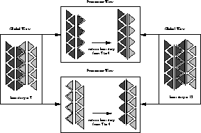
Figure 11.8: Illustration of a Parallel Collision During Load Balance. Each processor may take changes which decrease the boundary length, but the combined changes increase the boundary.

The problem with this parallel variant is, of course, that we are no longer doing the correct algorithm, since each processor is making changes without consulting the others. As noted in [Baiardi:89a], [Barajas:87a], [Braschi:90a], [Williams:86b], we have an algorithm which is highly parallel, but not particularly efficient. We should note that when the temperature is close to zero, the success rate of changes (ratio of accepted to proposed changes) falls to zero: Since a parallel collision depends on two successful changes, the parallel collision rate is proportional to the square of the low success rate, so that the effects of parallel collisions must be negligible at low temperatures.

One approach [Fox:88a] [Johnson:86a] to the parallel collision problem is rollback.  We make the changes in parallel, as above, then check to see if any parallel collisions have occurred, and if so, undo enough of the changes so that there are no collisions. While rollback ensures that the algorithm is carried out correctly, there may be a great deal of overhead, especially in a tightly coupled system at high temperature, where each change may collide with many others, and where most changes will be accepted. In addition, of course, rollback involves a large software and memory overhead since each change must be recorded in such a way that it can be rescinded, and a decision must be reached about which changes are to be undone.

For some cost functions and sets of changes, it may be possible to divide the possible changes into classes such that parallel changes within a class do not collide. An important model in statistical physics is the Potts model [Wu:82a], whose cost function is the same as the communication part of the load-balance cost function. If the underlying graph is a square lattice, the graph nodes may be divided into ``red'' and ``black'' classes, so called because the arrangement is like the red and black squares of a checkerboard . Then we may change all the red nodes or all the black nodes in parallel with no collisions.

Some highly efficient parallel simulated annealing algorithms have been implemented [Coddington:90a] for the Potts model  using clustering.  These methods are based on the locality of the Potts cost function: the change in cost function from a change in the color of a graph node depends only on the colors of the neighboring nodes of the graph. Unfortunately, the balance part of the cost function interferes with this locality in that widely separated (in terms of the Hamming distance) changes may collide, so these methods are not suitable for load balancing.

In this book, we shall use the simple collisional simulated annealing algorithm, making changes without checking for parallel collisions. Further work is required to invent and test more sophisticated parallel algorithms for simulated annealing, which may be able to avoid the degradation of performance caused by parallel collisions without unacceptable inefficiency from the parallelism [Baiardi:89a].

Clustering

Since the basic change made in the graph-coloring problem is to change the color of one node, a boundary can move at most one node per iteration. The boundaries between processors are diffusing toward their optimal configurations. A better change is to take a connected set of nodes which are the same color, and change the color of the entire set at once [Coddington:90a]. This is shown in Figure 11.9 where the cluster is chosen first by picking a random node; we then add nodes probabilistically to the cluster; in this case, the neighbor is added with probability 0.8 if it has the same color, and never if it has a different color. Once a neighbor has failed to be added, the cluster generation finishes. The coloring of the graph becomes optimal extremely quickly compared to the single color change method of Figure 11.6.

  
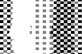
Figure: Same as Figure 11.6, Except the Basic Move Is to Change the Color of a Connected Cluster of Nodes.

Figure 11.10 shows the clustered simulated annealing running in parallel, where 16 clusters are chosen simultaneously. The performance is degraded, but still better than Figure 11.7, which is parallel but with single color changes.

  
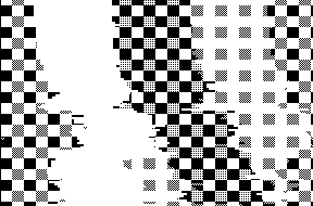
Figure: Same as Figure 11.7, Except That the Cluster Method Is Being Carried Out in Parallel by 16 Processors.

Summary of the Algorithm

The annealing algorithm as presented so far requires that several parameters be chosen for tuning, which are in italic font in the description below.

First, we pick the initial coloring of the graph so that each graph node takes a color corresponding to the processor in which it currently resides. We form a population table, of which each processor has a copy of , the number of nodes which have color q. We pick a value for , the importance of communication.

We pick a maximum temperature and the number of stages during which the temperature is to be reduced to zero. Each stage consists of a number of changes to the graph coloring which may be accepted or rejected, with no communication between the processors. At the end of the stage, each processor has a different idea of the population table, and the colors of neighboring graph nodes which are in different processors, because each processor has made changes without knowledge of the others. At the end of the stage, the processors communicate to update the population tables and local neighbor information so that each processor has up-to-date information. Each stage consists of either having a given number of accepted changes, or a given number of rejected changes, whichever comes first, followed by a loosely synchronous communication between processors.

Each trial move within a stage consists of looking for a cluster of uniform color, choosing a new color for the cluster, evaluating the change in cost function, and using the Metropolis  criterion to decide whether to accept it. The cluster is chosen by first picking a random graph node as a seed, and probabilistically forming a cluster. Neighboring nodes are added to the cluster with a given cluster probability if they are the same color as the seed and reside in the same processor.

The proposed new color for the cluster is chosen to be either random with given seed probability, or a random color chosen from the set of neighbors of the cluster. The Metropolis criterion is then used to decide if the color change is to be accepted, and if so, the local copy of the population table is updated.