This example program demonstrates the basic requirements to call a ScaLAPACK routine -- initializing the process grid, assigning the matrix to the processes, calling the ScaLAPACK routine, and releasing the process grid. For further details on each of these steps, please refer to section 2.4.
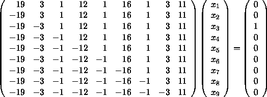
This example program solves the ![]() system of linear
equations given by
system of linear
equations given by

using the ScaLAPACK driver routine PDGESV.
The ScaLAPACK routine PDGESV solves a system of linear
equations ![]() , where the coefficient matrix (denoted by A) and the
right-hand-side matrix (denoted by B) are real, general distributed matrices.
The coefficient matrix A is distributed as depicted below, and for simplicity,
we shall solve the system for one right-hand side (NRHS=1); that is, the matrix
B is a vector. The third element of the matrix B is equal to 1, and all other
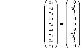
elements are equal to 0. After solving this system of equations, the solution
vector X is given by
, where the coefficient matrix (denoted by A) and the
right-hand-side matrix (denoted by B) are real, general distributed matrices.
The coefficient matrix A is distributed as depicted below, and for simplicity,
we shall solve the system for one right-hand side (NRHS=1); that is, the matrix
B is a vector. The third element of the matrix B is equal to 1, and all other
elements are equal to 0. After solving this system of equations, the solution
vector X is given by
Let us assume that the matrix A is partitioned and distributed as denoted
in figure 4.6; that is, we have chosen
the row and column block sizes as MB=NB=2, and the matrix is distributed
on a 2 ![]() 3 process grid (
3 process grid (![]() ,
,![]() ). The partitioning
and distribution of our example matrix A is represented in
figures 2.1 and 2.2, where, to aid visualization,
we use the notation s=19, c=3, a=1, l=12, p=16, and k=11.
). The partitioning
and distribution of our example matrix A is represented in
figures 2.1 and 2.2, where, to aid visualization,
we use the notation s=19, c=3, a=1, l=12, p=16, and k=11.
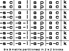
Figure 2.1: Partitioning of global matrix A (s=19;c=3;a=1;l=12;p=16;k=11)
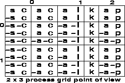
Figure 2.2: Mapping of matrix A onto process grid (![]() ,
,![]() ).
For example, note that process (0,0) contains a local array
of size A(5,4).
).
For example, note that process (0,0) contains a local array
of size A(5,4).
The partitioning and distribution of our example matrix B are demonstrated in figure 2.3.
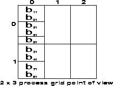
Figure 2.3: Mapping of matrix B onto process grid (![]() ,
,![]() )
)
Note that matrix B is distributed only in column 0 of the process grid. All other columns in the process grid possess an empty local portion of the matrix B.
On exit from PDGESV, process (0,0) contains (in the global view)
the global vector X and (in the local view) the local array B given by

and process (1,0) contains (in the global view) the global vector X and
(in the local view) local array B given by

The normalized residual check
![]()
is performed on the solution to verify the accuracy of the results.
For more information on the BLACS routines called in this program, please refer to section 2.4, Appendix D.3, [54], and the BLACS homepage (http://www.netlib.org/blacs/index.html). Further details of the matrix distribution and storage scheme can be found in section 2.3.2, figure 4.6, and table 4.8. Complete details on matrix distribution can be found in Chapter 4 and details of the array descriptors can be found in section 4.3.2. For a more flexible and memory efficient example program, please refer to Appendix C.1.