

Next: Array Descriptor for In-core
Up: In-core Dense Matrices
Previous: The Two-dimensional Block-Cyclic Distribution
The block-cyclic distribution scheme
is a mapping of a set of blocks onto
the processes. The previous section
informally described this mapping as
well as some of its properties. To
be complete, we must now explain how
the blocks that are mapped to the
same process are arranged and
stored in the local process memory.
In other words, we shall describe
the precise mapping that associates
to a matrix entry identified by its
global indexes the coordinates of
the process that owns it and its
local position within that process's
memory.
Suppose we have an array of length
N to be stored on P processes.
By convention, the array entries
are numbered 1 through N and
the processes are numbered 0
through P-1. First, the array
is divided into contiguous blocks
of size NB. When NB does not
divide N evenly, the last block
of array elements will only contain
 entries instead
of NB. By convention, these blocks
are numbered starting from zero and
dealt out to the processes like a
deck of cards. In other words, if
we assume that the process 0
receives the first block, the
  block is assigned to the process of
coordinate
  . The
blocks assigned to the same process
are stored contiguously in memory.
The mapping of an array entry
globally indexed by I is defined
by the following analytical equation:

where I is a global index in the
array, l is the local block coordinate
into which this entry resides, p
is the coordinate of the process
owning that block, and finally x
is the coordinate within that block
where the global array entry of
index I is to be found. It is
then fairly easy to establish the
analytical relationship between
these variables. One obtains:

These equations allow to determine
the local information, i.e. the
local index  as
well as the process coordinate
p corresponding to a global entry
identified by its global index I
and conversely. Table 4.3
illustrates this mapping for the block
layout when P=2 and N=16, i.e.,
NB=8. At most one block is assigned
to each process.

Table 4.3: One-dimensional block mapping example for P=2 and N=16
This example of the one-dimensional
block distribution mapping can be
expressed in HPF
by using the following statements:
      REAL :: X( N )
!HPF$ PROCESSORS PROC( P )
!HPF$ DISTRIBUTE X( BLOCK( NB ) ) ONTO PROC
Table 4.4 illustrates
Equation 4.1 for
the cyclic layout, i.e., NB=1
when P=2 and N=16.

Table 4.4: One-dimensional cyclic mapping example for P=2
and N=16
This example of the one-dimensional cyclic
distribution mapping can be expressed in
HPF by using the
following statements:
      REAL :: X( N )
!HPF$ PROCESSORS PROC( P )
!HPF$ DISTRIBUTE X( CYCLIC ) ONTO PROC
Table 4.5 illustrates
Equation 4.1 for
the block-cyclic layout when P=2,
NB=3 and N=16.

Table 4.5: One-dimensional block-cyclic mapping example for
P=2, NB=3 and N=16
This example of the one-dimensional cyclic
distribution mapping can be expressed in
HPF by using the
following statements:
      REAL :: X( N )
!HPF$ PROCESSORS PROC( P )
!HPF$ DISTRIBUTE X( CYCLIC( NB ) ) ONTO PROC
There is in fact no real
reason to always deal out
the blocks starting with
the process 0. In fact,
it is sometimes useful to
start the data distribution
with the process of arbitrary
coordinate SRC, in which case
Equation 4.1
becomes:

Table 4.6
illustrates Equation 4.2
for the block-cyclic layout when  ,
,
 ,
,  and
and  .
.

Table 4.6: One-dimensional block-cyclic mapping example for
P=2, SRC=1, NB=3 and N=16
This example
of the one-dimensional
block-cyclic distribution
mapping can be expressed
in HPF
by using the following statements:
      REAL :: X( N )
!HPF$ PROCESSORS PROC( P )
!HPF$ TEMPLATE T( N + P*NB )
!HPF$ DISTRIBUTE T( CYCLIC( NB ) ) ONTO PROC
!HPF$ ALIGN X( I ) WITH T( SRC*NB + I )
In the two-dimensional case,
assuming the matrix is partitioned
in  blocks and that
the first block is given to the
process of coordinates (RSRC, CSRC),
the analytical formula given above for
the one-dimensional case are simply
reused independently in each dimension
of the
  process grid.
For example, the matrix entry (I,J)
is thus to be found in the process
of coordinates
  within
the local (l,m) block at the
position (x,y) given by:

These formula specify how an  by
by  matrix A is mapped and stored on the
process grid. It is first decomposed
into
  by
by  blocks starting at its upper left
corner. These blocks are then
uniformly distributed across the
process grid in a cyclic manner.
Every process owns a collection
of blocks, which are contiguously
stored by column in a two-dimensional
``column major'' array.
This local storage convention
allows the ScaLAPACK software to
use efficiently the local memory
hierarchy by calling the BLAS on
subarrays that may be larger than
a single  by
by  block.
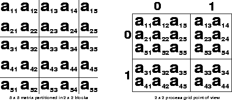
We present in figure 4.5
the mapping of a 5
 5
matrix partitioned into 2
 2
blocks mapped onto a 2
 2
process grid (i.e.,
  ,
,  ,
and
,
and  ). The local entries of
every matrix column are contiguously stored
in the processes' memories.

Figure 4.6: A  matrix decomposed into
  blocks mapped onto a
  process grid
In figure 4.5, the process
of coordinates (0,0) owns four blocks.
The matrix entries of the global columns
1, 2 and 5 are contiguously stored in
that process's memory. Finally, these
columns are themselves continuously stored
forming a conventional two-dimensional
local array. In that local array A,
the entry A(2,3) contains the value
of the global matrix entry  .
This example would be expressed in
HPF as:
      REAL :: A( 5, 5 )
!HPF$ PROCESSORS PROC( 2, 2 )
!HPF$ DISTRIBUTE A( CYCLIC( 2 ), CYCLIC( 2 ) ) ONTO PROC
Determining the number of
rows or columns of a global
dense matrix that a specific
process receives is an
essential task for the
user. ScaLAPACK provides
a tool routine, NUMROC,
to perform this function.
The notation LOC ()
and LOC
 () is used
to reflect these local
quantities throughout the
leading comments of the
source code and is reflected
in the sample argument
description in section 4.3.5.
The values of LOC
 ()
and LOC
 () computed
by NUMROC are precise calculations.
However, if users want a
general idea of the size
of a local array, they can
perform the following ``back
of the envelope'' calculation
to receive an upper bound on
the quantity.
An upper bound on the value of LOC () can be calculated as:

or equivalently as

Similarly, an upper bound on the value of
LOC () can be calculated as

or equivalently as

Note that this calculation can
yield a gross overestimate of
the amount of space actually
required.


Next: Array Descriptor for In-core
Up: In-core Dense Matrices
Previous: The Two-dimensional Block-Cyclic Distribution
Susan Blackford
Tue May 13 09:21:01 EDT 1997


