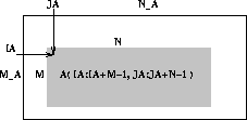
Figure 4.7: Global view of the matrix operands
As previously mentioned, the ScaLAPACK routines that solve dense linear systems and eigenvalue problems assume that all global arrays are distributed in a one- or two-dimensional block cyclic fashion. After a global vector or matrix has been block-cyclicly distributed over a process grid, the user may choose to perform an operation on a portion of the global matrix. This subset of the global matrix is referred to as a ``submatrix'' and is referenced through the use of six arguments in the calling sequence: the number of rows of the submatrix M, the number of columns of the submatrix N, the local array A containing the global array, the row index IA, the column index JA and the array descriptor of the global array DESCA. This argument convention allows for a global view of the matrix operands and the global addressing of distributed matrices as illustrated in figure 4.7. This scheme allows the complete specification of the submatrix A(IA:IA+M-1,JA:JA+N-1) on which to be operated.

Figure 4.7: Global view of the matrix operands
The description of a global dense subarray consists of (M, N, A, IA, JA, DESCA)
The names of the row and column indices for the global array have the form I<array_name> and J<array_name> , respectively. The array descriptor has a name of the form DESC<array_name> . The length of the array descriptor is specified by DLEN_ and varies according to the descriptor type DTYPE_.
Included in the leading comments of each subroutine (immediately preceding the Argument section), is a brief note describing the array descriptor and some commonly used expressions in calculating workspace.
The style of the argument descriptions for dense matrices is illustrated by the following example. As previously mentioned, the notations x_ used in the entries of the array descriptor denote the attributes of a global array. For readability of the code, we have associated symbolic names for the descriptor entries. For example, M_ denotes the number of rows and M_A specifically denotes the number of rows in global matrix A. Complete details can be found in section 4.3.3.
The description of each argument gives
These dimensions are often expressed in terms of
LOC![]() () and LOC
() and LOC![]() () calculations. For
further details, please refer to section 4.3.2.
() calculations. For
further details, please refer to section 4.3.2.