In this section, we consider the data layout of dense matrices on distributed-memory machines, with the goal of making dense matrix computations as efficient as possible. We shall discuss a sequence of data layouts, starting with the most simple, obvious, and inefficient one and working up to the complicated but efficient ScaLAPACK ultimately uses. Even though our justification is based on Gaussian elimination, analysis of many other algorithms has led to the same set of layouts. As a result, these layouts have been standardized as part of the High Performance Fortran standard [91], with corresponding data declarations as part of that language.
The two main issues in choosing a data layout for dense matrix computations are
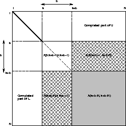
It will help to remember the pictorial
representation of Gaussian elimination
below. As the algorithm proceeds, it
works on successively smaller square
southeast corners of the matrix. In
addition, there is extra Level 2 BLAS
work to factorize the submatrix
![]() .
.

Figure 4.2: Gaussian elimination using Level 3 BLAS
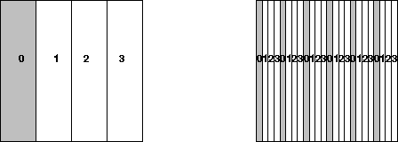
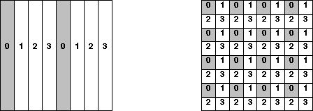
For convenience we will number the processes from 0 to P-1, and matrix columns (or rows) from 1 to N. The following two figures shows a sequence of data layouts we will consider. In all cases, each submatrix is labeled with the number of the process (from 0 to 3) that contains it. Process 0 owns the shaded submatrices.
Consider the layout illustrated on the left of figure 4.3, the one-dimensional block column distribution. This distribution

Figure 4.3: The one-dimensional block and cyclic column distributions
assigns a block of contiguous columns
of a matrix to successive processes.
Each process receives only one block
of columns of the matrix. Column k
is stored on process ![]() where
where ![]() is the maximum number of
columns stored per process. In the
figure N=16 and P=4. This layout
does not permit good load balancing
for the above Gaussian elimination
algorithm because as soon as the
first tc columns are complete,
process 0 is idle for the rest
of the computation. The transpose
of this layout, the one-dimensional
block row distribution, has a similar
shortfall for dense computations.
is the maximum number of
columns stored per process. In the
figure N=16 and P=4. This layout
does not permit good load balancing
for the above Gaussian elimination
algorithm because as soon as the
first tc columns are complete,
process 0 is idle for the rest
of the computation. The transpose
of this layout, the one-dimensional
block row distribution, has a similar
shortfall for dense computations.
The second layout illustrated on the right of
figure 4.3, the one-dimensional
cyclic column distribution, addressed this
problem by assigning column k to process
(k-1) mod P. In the figure, N=16 and P=4.
With this layout, each process owns approximately
![]() of the square southeast corner of the
matrix, so the load balance is good. However,
since single columns (rather than blocks) are
stored, we cannot use the Level 2 BLAS to
factorize
of the square southeast corner of the
matrix, so the load balance is good. However,
since single columns (rather than blocks) are
stored, we cannot use the Level 2 BLAS to
factorize ![]() and may not be
able to use the Level 3 BLAS to update
and may not be
able to use the Level 3 BLAS to update
![]() . The transpose of this
layout, the one-dimensional cyclic
row distribution, has a similar shortfall.
. The transpose of this
layout, the one-dimensional cyclic
row distribution, has a similar shortfall.
The third layout shown on the left of
figure 4.4, the
one-dimensional block-cyclic
column distribution, is a compromise
between the distribution schemes shown
in figure 4.3. We choose a
block size NB, divide the columns
into groups of size NB, and distribute
these groups in a cyclic manner. This
means column k is stored in process
![]() .
In fact, this layout includes the first
two as the special cases,
.
In fact, this layout includes the first
two as the special cases, ![]() and NB=1, respectively.
In the figure N=16, P=4 and NB=2.
For NB larger than 1, this has a
slightly worse balance than the
one-dimensional cyclic column
distribution, but can use the
Level 2 BLAS and Level 3 BLAS
for the local computations.
For NB less than tc, it
has a better load balance than
the one-dimensional block column
distribution, but can call the BLAS
only on smaller subproblems. Hence,
it takes less advantage of the local
memory hierarchy. Moreover, this
layout has the disadvantage that
the factorization of
and NB=1, respectively.
In the figure N=16, P=4 and NB=2.
For NB larger than 1, this has a
slightly worse balance than the
one-dimensional cyclic column
distribution, but can use the
Level 2 BLAS and Level 3 BLAS
for the local computations.
For NB less than tc, it
has a better load balance than
the one-dimensional block column
distribution, but can call the BLAS
only on smaller subproblems. Hence,
it takes less advantage of the local
memory hierarchy. Moreover, this
layout has the disadvantage that
the factorization of ![]() will take place on one process (in the
natural situation where column blocks
in the layout correspond to column
blocks in Gaussian elimination),
thereby representing a serial bottleneck.
will take place on one process (in the
natural situation where column blocks
in the layout correspond to column
blocks in Gaussian elimination),
thereby representing a serial bottleneck.

Figure 4.4: The one-dimensional block-cyclic column- and the two-dimensional
block-cyclic distributions
This serial bottleneck is eased by the
fourth layout shown on the right of
figure 4.4, the
two-dimensional block cyclic distribution.
Here, we think of our P processes arranged
in a ![]()
![]()
![]() rectangular
array of processes, indexed in a two-dimensional
fashion by
rectangular
array of processes, indexed in a two-dimensional
fashion by ![]() , with
, with ![]() and
and ![]() . All the processes
. All the processes
![]() with a fixed
with a fixed ![]() are referred
to as process column
are referred
to as process column ![]() . All the processes
. All the processes
![]() with a fixed
with a fixed ![]() are referred
to as process row
are referred
to as process row ![]() . Thus, this layout
includes all the previous layouts, and their
transposes, as special cases. In the figure,
N=16, P=4,
. Thus, this layout
includes all the previous layouts, and their
transposes, as special cases. In the figure,
N=16, P=4, ![]() , and MB=NB=2.
This layout permits
, and MB=NB=2.
This layout permits ![]() -fold parallelism
in any column, and calls to the Level 2 BLAS
and Level 3 BLAS on local subarrays. Finally,
this layout also features good scalability
properties as shown in [61].
-fold parallelism
in any column, and calls to the Level 2 BLAS
and Level 3 BLAS on local subarrays. Finally,
this layout also features good scalability
properties as shown in [61].
The two-dimensional block cyclic distribution scheme is the data layout that is used in the ScaLAPACK library for dense matrix computations.