The analysis is given for the Cayley transform only, though shift-and-invert could be used as well. The reasons are threefold. First, the shift-and-invert Arnoldi method and the Cayley transform Arnoldi method produce the same Ritz vectors. Second, it makes a link with the (Jacobi) Davidson methods easier to establish. Third, the Cayley transform leads to a more natural approach to the problem.
In the Arnoldi method applied to the Cayley transform,
![]() , we must
solve a
sequence of linear systems
, we must
solve a
sequence of linear systems
By putting all the ![]() for
for
![]() together in
together in
![]() ,
,
![]() in
in ![]() and
and ![]() in
in ![]() , we obtain
, we obtain
Note that for a fixed ![]() and
and ![]() ,
,
![]() depends on
depends on ![]() and the way each of the linear systems (11.2) are solved.
When (11.2) is
solved by a preconditioner
and the way each of the linear systems (11.2) are solved.
When (11.2) is
solved by a preconditioner ![]() or a stationary linear system solver, i.e.,
or a stationary linear system solver, i.e.,
![]() for
for
![]() , then
, then
![]() is independent of
is independent of ![]() and
and
![]() and so is
and so is
![]() .
.
Eigenpairs are computed from
![]() .
In Arnoldi's method, this happens by the Hessenberg matrix that arises
from the
orthogonalization of
.
In Arnoldi's method, this happens by the Hessenberg matrix that arises
from the
orthogonalization of ![]() ; in the Davidson method, one uses the
projection
with
; in the Davidson method, one uses the
projection
with ![]() and
and ![]() , e.g.,
, e.g.,
![]() .
.
![]() contains the eigenvectors associated
with the
well-separated extreme eigenvalues of
contains the eigenvectors associated
with the
well-separated extreme eigenvalues of
![]() .
This is a perturbed
.
This is a perturbed
![]() , so the relation with
, so the relation with ![]() is
partially
lost, and accurately computing eigenpairs of
is
partially
lost, and accurately computing eigenpairs of ![]() may be
difficult.
To see which parameters play a role in this perturbation,
from Theorems 4.3 and 4.4 in [323], it can be shown that
if
may be
difficult.
To see which parameters play a role in this perturbation,
from Theorems 4.3 and 4.4 in [323], it can be shown that
if
![]() has distinct eigenvalues,
then for each eigenpair
has distinct eigenvalues,
then for each eigenpair ![]() of
of
![]() there is an eigenpair
there is an eigenpair ![]() of
of
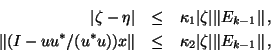
![]() such that
such that
This section can be concluded as follows.
The remaining question is now how to compute the eigenpairs of
![]() or
how to exploit them for computing eigenpairs of
or
how to exploit them for computing eigenpairs of
![]() .
In §11.2.3 and §11.2.4,
we discuss the Rayleigh-Ritz technique; i.e.,
eigenpairs are computed from the orthogonal projection of
.
In §11.2.3 and §11.2.4,
we discuss the Rayleigh-Ritz technique; i.e.,
eigenpairs are computed from the orthogonal projection of
![]() on the
on the
![]() .
In §11.2.7, the eigenpairs are computed from the
eigenpairs of
.
In §11.2.7, the eigenpairs are computed from the
eigenpairs of
![]() directly by use of the rational Krylov recurrence relation.
§11.2.6 presents a Lanczos algorithm that uses the
recurrence relation for the eigenvectors and the Rayleigh-Ritz projection
for the eigenvalues.
directly by use of the rational Krylov recurrence relation.
§11.2.6 presents a Lanczos algorithm that uses the
recurrence relation for the eigenvectors and the Rayleigh-Ritz projection
for the eigenvalues.
Note that ![]() and
and ![]() cannot be chosen too far away from each other.
Suppose the eigenvalue
cannot be chosen too far away from each other.
Suppose the eigenvalue ![]() is wanted. From the conclusion given
above, the convergence is faster when
is wanted. From the conclusion given
above, the convergence is faster when ![]() is
chosen close to
is
chosen close to ![]() , and the computed eigenvalue can only be
accurate when
, and the computed eigenvalue can only be
accurate when
![]() is close to
is close to ![]() .
In theory, one could select
.
In theory, one could select ![]() , which is usually used in
the Davidson method.
Since
, which is usually used in
the Davidson method.
Since
![]() in that case, there is a high risk of stagnation in the
latter method.
A robust selection is used in the Jacobi-Davidson method, which we
discuss
in §11.2.5.
in that case, there is a high risk of stagnation in the
latter method.
A robust selection is used in the Jacobi-Davidson method, which we
discuss
in §11.2.5.