The Jacobi-Davidson method is discussed in §7.12.
The Jacobi-Davidson method differs from the Davidson method in that the
linear
system to be solved is projected onto the space orthogonal to the current
Ritz vector.
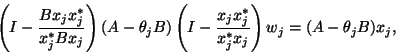
This leads to the solution of the correction equation
In words, the solution ![]() of the correction equation is obtained by
the
action of the Cayley transform
of the correction equation is obtained by
the
action of the Cayley transform
![]() to the most
recent
Ritz vector.
Example 11.2.1 in [411] shows that
to the most
recent
Ritz vector.
Example 11.2.1 in [411] shows that ![]() tends to zero on
convergence.
Both pole and zero of the Cayley transform lie close to the desired
eigenvalue.
This meets the conditions for good matching between
eigenvectors of
tends to zero on
convergence.
Both pole and zero of the Cayley transform lie close to the desired
eigenvalue.
This meets the conditions for good matching between
eigenvectors of ![]() and
and
![]() ,
motivated at the end of §11.2.2.
,
motivated at the end of §11.2.2.
The following observation is a bit funny.
Since
![]() ,
when
,
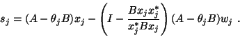
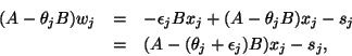
when ![]() , we have from
, we have from
![]() that
that