 , and the
following unusual exponential singularity in the correlation length and
magnetic susceptibility:


The XY (or O(2)) model consists of a set of continuous
valued spins regularly arranged on a two-dimensional square lattice.
Fifteen years ago, Kosterlitz and Thouless (KT) predicted that this system would undergo a phase
transition as one changed from a low-temperature
spin wave phase to a high-temperature phase with unbound vortices. KT
predicted an approximate transition temperature,  , and the
following unusual exponential singularity in the correlation length and
magnetic susceptibility:
with

where  and the correlation function exponent
  is defined
by the relation
  .
.
Our simulation [Gupta:88a] was done on the 128-node FPS
(Floating Point Systems) T-Series hypercube at Los Alamos. FPS
software allowed the use of C with a software model similar
(communication implemented by subroutine call) to that used on the
hypercubes at Caltech. Each FPS node is built around Weitek
floating-point units, and we achieved  per node in this
application. The total machine ran at
  , or at about
twice the performance of one processor of a CRAY X-MP for
this application. We use a 1-D torus topology for communications,
with each node processing a fraction of the rows. Each row is divided
into red/black alternating sites of spins and the vector loop is over a
given color. This gives a natural data structure of (
 )
words for lattices of size
  . The internode
communications, in both lattice update and measurement of observables,
can be done asynchronously and are a negligible overhead.

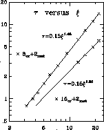
Figure 4.19: Autocorrelation Times for the XY Model
Previous numerical work was unable to confirm the KT theory, due to limited
statistics and small lattices. Our high-statistics simulations are done on
 ,
,  ,
,  , and
, and  lattices using a combination of
over-relaxed and Metropolis algorithms which
decorrelates as
  . (For comparison, a
Metropolis algorithm decorrelates as
  .) Each
configuration represents
  over-relaxed sweeps through the
lattice followed by
  Metropolis sweeps. Measurement of
observables is made on every configuration. The over-relaxed algorithm
consists of reflecting the spin at a given site about
  , where
 is the sum of the nearest-neighbor spins, that is,

This implementation [Creutz:87a], [Brown:87a] of the
over-relaxed algorithm is microcanonical, and it reduces critical
slowing down even though it is a local algorithm. The ``hit'' elements
for the Metropolis algorithm are generated as  , where
 is a uniform random number in the
interval
  , and
, and  is adjusted to
give an acceptance rate of 50 to 60 percent. The Metropolis hits make
the algorithm ergodic, but their effectiveness is limited to local
changes in the energy. In Figure 4.19, we show the
autocorrelation time
  vs. the correlation length
  ; for
; for
 ,
,  we extract
  , and
for
  ,
,  we get
  .
.

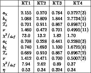
Table 4.7: Results of the XY Model Fits: (a)  in T, and (b)
  in T Assuming the KT Form. The fits KT1-3 are pseudominima while KT4 is
the true minimum. All data points are included in the fits and we give the
 for each fit and an estimate of the exponent
  .
.
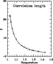
We ran at 14 temperatures near the phase transition and made unconstrained fits to all 14 data points (four parameter fits according to Equation 4.24), for both the correlation length (Figure 4.20) and susceptibility (Figure 4.21). The key to the interpretation of the data is the fits. We find that fitting programs (e.g., MINUIT, SLAC) move incredibly slowly towards the true minimum from certain points (which we label spurious minima), which, unfortunately, are the attractors for most starting points. We found three such spurious minima (KT1-3) and the true minimum KT4, as listed in Table 4.7.

Figure 4.20: Correlation Length for the XY Model

Figure 4.21: Susceptibility for the XY Model
Thus, our data was found to be in excellent agreement with the KT theory and,
in fact, this study provides the first direct measurement of  from both
 and
and  data that is consistent with the KT predictions.


