


Next: 4.5 An Automata Model
Up: 4.4 Spin Models
Previous: 4.4.4 XY Model
The XY model is the simplest O(N) model, having N=2, the O(N) model
being a set of rotors (N-component continuous valued spins) on an
N-sphere. For  , this model is asymptotically free
[Polyakov:75a], and for N=3, there exist so called instanton
solutions. Some of these properties are analogous to those of gauge
theories in four dimensions; hence, these models are interesting. In
particular, the O(3) model in two dimensions should
shed some light on the asymptotic freedom of QCD (SU(3)) in four
dimensions. The predictions of the renormalization group for the
susceptibility
  and inverse correlation length (i.e., mass gap)
m in the O(3) model are [Brezin:76a]

and

respectively. If m and  vary according to these equations,
without the correction of order
  , they are said to follow
asymptotic scaling. Previous work was able
to confirm that this picture is qualitatively correct, but was not able
to probe deep enough in the area of large correlation lengths to obtain
good agreement.
The combination of the over-relaxed algorithm and the computational
power of the FPS T-Series allowed us to simulate lattices of sizes up
to  . We were thus able to simulate at coupling constants that
correspond to correlation lengths up to 300, on lattices where
finite-size effects are negligible. We were also able to gather large
statistics and thus obtain small statistical errors. Our simulation is
in good agreement with similar cluster calculations
[Wolff:89b;90a]. Thus, we have validated and
extended these results in a regime where our algorithm is the only
known alternative to clustering.
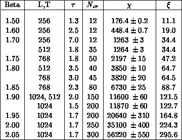
Table 4.8: Coupling Constant, Lattice Size, Autocorrelation Time, Number of
Overrelaxed Sweeps, Susceptibility, and Correlation Length for the O(3)
Model
We have made extensive runs at 10 values of the coupling constant. At the
lowest  , several hundred thousand sweeps were collected, while for the
largest values of
  , between 50,000 and 100,000 sweeps were made.
Each sweep consists of between 10 iterations through the lattice at the
former end and 150 iterations at the latter. The statistics we have gathered
are equivalent to about 200 days, use of the full 128-node FPS machine.
Our results for the correlation length and susceptibility for each
coupling  and lattice size are shown in Table 4.8.
The autocorrelation times are also shown. The quantities measured on
different-sized lattices at the same
  agree, showing that the
infinite volume limit has been reached.
To compare the behavior of the correlation length and susceptibility
with the asymptotic scaling predictions, we use the ``correlation
length defect''  and ``susceptibility defect''
 , which are defined as follows:
  ,
,  ,
so that asymptotic scaling is seen if
  ,
,  go to constants as
  . These defects are shown
in Figures 4.22 and 4.23, respectively. It
is clear that asymptotic scaling does not set in for
  , but
it is not possible to draw a clear conclusion for
  -though
the trends of the last two or three points may be toward constant behavior.
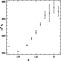
Figure 4.22: Correlation Length Defect Versus the Coupling Constant for the O(3)
Model
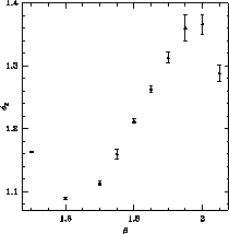
Figure 4.23: Susceptibility Defect Versus the Coupling Constant for the O(3) Model
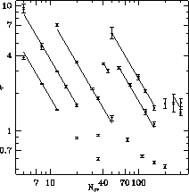
Figure 4.24: Decorrelation Time  Versus Number of Over-relations Sweeps
 for Different Values of
We gauged the speed of the algorithm in producing statistically independent
configurations by measuring the autocorrelation time  . We used this to
estimate the dynamical critical exponent z, which is defined by
  . For constant
  , our fits give
  . However,
we discovered that by increasing
  in rough proportion to
  , we
can improve the performance of the algorithm significantly. To compare the
speed of decorrelation between runs with different
  , we define a new
quantity, which we call ``effort,''
  . This measures
the computational effort expended to obtain a decorrelated configuration. We
define a new exponent
  from
from  , where
  is chosen to keep
  constant. We also found that the behavior of
the decorrelation time can be approximated over a good range by

A fit to the set of points ( ,
,  ,
,  ) gives
 ,
,  . Thus,
  is
significantly lower than z. Figure 4.24 shows
  versus
 , with the fits shown as solid lines.


Next: 4.5 An Automata Model
Up: 4.4 Spin Models
Previous: 4.4.4 XY Model
Guy Robinson
Wed Mar 1 10:19:35 EST 1995
 , this model is asymptotically free
[Polyakov:75a], and for N=3, there exist so called instanton
solutions. Some of these properties are analogous to those of gauge
theories in four dimensions; hence, these models are interesting. In
particular, the O(3) model in two dimensions should
shed some light on the asymptotic freedom of QCD (SU(3)) in four
dimensions. The predictions of the renormalization group for the
susceptibility
  and inverse correlation length (i.e., mass gap)
m in the O(3) model are [Brezin:76a]


 vary according to these equations,
without the correction of order
  , they are said to follow
asymptotic scaling.
 . We were thus able to simulate at coupling constants that
correspond to correlation lengths up to 300, on lattices where
finite-size effects are negligible. We were also able to gather large
statistics and thus obtain small statistical errors. Our simulation is
in good agreement with similar cluster calculations
[Wolff:89b;90a]. Thus, we have validated and
extended these results in a regime where our algorithm is the only
known alternative to clustering.

 , several hundred thousand sweeps were collected, while for the
largest values of
  , between 50,000 and 100,000 sweeps were made.
Each sweep consists of between 10 iterations through the lattice at the
former end and 150 iterations at the latter. The statistics we have gathered
are equivalent to about 200 days, use of the full 128-node FPS machine.
 and lattice size are shown in Table
  agree, showing that the
infinite volume limit has been reached.
 and ``susceptibility defect''
 , which are defined as follows:
  ,
,  ,
so that asymptotic scaling is seen if
  ,
,  go to constants as
  . These defects are shown
in Figures
  , but
it is not possible to draw a clear conclusion for
  -though
the trends of the last two or three points may be toward constant behavior.


 Versus Number of Over-relations Sweeps
 for Different Values of
 . We used this to
estimate the dynamical critical exponent z, which is defined by
  . For constant
  , our fits give
  . However,
we discovered that by increasing
  in rough proportion to
  , we
can improve the performance of the algorithm significantly. To compare the
speed of decorrelation between runs with different
  , we define a new
quantity, which we call ``effort,''
  . This measures
the computational effort expended to obtain a decorrelated configuration. We
define a new exponent
  from
from  , where
  is chosen to keep
  constant. We also found that the behavior of
the decorrelation time can be approximated over a good range by

 ,
,  ,
,  ) gives
 ,
,  . Thus,
  is
significantly lower than z. Figure
  versus
 , with the fits shown as solid lines.