 , which can take q different values, and whose
Hamiltonian is


The q-state Potts model [Potts:52a] consists of a
lattice of spins  , which can take q different values, and whose
Hamiltonian is

For q=2, this is equivalent to the Ising model. The Potts model is thus a simple extension of the Ising model; however, it has a much richer phase structure, which makes it an important testing ground for new theories and algorithms in the study of critical phenomena [Wu:82a].
Monte Carlo simulations of Potts models have
traditionally used local algorithms such as that of
Metropolis, et al. [Metropolis:53a], however,
these algorithms have the major drawback that near a phase transition,
the autocorrelation time (the number of sweeps needed to generate a
statistically independent configuration) increases approximately as
 , where L is the linear size of the lattice. New algorithms
have recently been developed that dramatically reduce this ``critical
slowing down'' by updating clusters of
spins at a time (these algorithms are described in
Section 12.6). The original cluster algorithm of Swendsen and
Wang (SW) was implemented for the Potts model [Swendsen:87a], and
there is a lot of interest in how well cluster algorithms perform for
this model. At present, there are very few theoretical results known
about cluster algorithms, and theoretical
advances are most likely to come from first studying the simplest
possible models.
We have made a high statistics study of the SW algorithm and the single
cluster Wolff algorithm [Wolff:89b], as well as a number of variants of
these algorithms, for the q=2 and q=3 Potts models in two dimensions
[Baillie:90n]. We measured the autocorrelation time  in the
energy (a local operator) and the magnetization (a global one) on lattice
sizes from
  to
to  . About 10 million sweeps were required for each
lattice size in order to measure autocorrelation times to within about 1 percent.
From these values, we can extract the dynamic critical exponent z, given
by
  , where
  is measured at the infinite volume
critical point (which is known exactly for the two-dimensional Potts model).
The simulations were performed on a number of different parallel
computers. For lattice sizes of  or less, it is possible to run
independent simulations on each processor of a parallel machine,
enabling us to obtain 100 percent efficiency by running 10 or 20 runs
for each lattice size in parallel, using different random
number streams. These calculations were done
using a 32-processor Meiko Computing Surface, a
20-processor Sequent Symmetry, a 20-processor
Encore Multimax, and a 96-processor BBN GP1000
Butterfly , as well as a network of SUN
workstations. The calculations ook approximately 15,000
processor-hours. For the largest lattice sizes,
  and
and  , a
parallel cluster algorithm was required, due to the large amount of
calculation (and memory) required. We have used the
self-labelling algorithm described in
Section 12.6, which gives fairly good efficiencies of about
70 percent on the machines we have used (an nCUBE-1 and a Symult
S2010), by doing multiple runs of 32 nodes each for the
  lattice, and 64 nodes for
  . Since this problem does not
vectorize, using all 512 nodes of the nCUBE gives a performance
approximately five times that of a single processor
CRAY X-MP, while all 192 nodes of the Symult is equivalent
to about six CRAYs. The calculations on these machines have so far
taken about 1000 hours.
Results for the autocorrelation times of the energy for the Wolff and SW
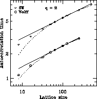
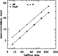
algorithms are shown in Figure 4.17 for q=2 and
Figure 4.18 for q=3. As can be seen, the Wolff algorithm has
smaller autocorrelation times than SW. However, the dynamical critical
exponents for the two algorithms appear to be identical, being approximately
 and
and  for q=2 and q=3 respectively (shown as
straight lines in Figures 4.17 and 4.18),
compared to values of approximately 2 for the standard Metropolis
algorithm.

Figure 4.17: Energy Autocorrelation Times, q=2

Figure 4.18: Energy Autocorrelation Times, q=3
Burkitt and Heermann [Heermann:90a] have suggested that the increase in
the autocorrelation time is a logarithmic one, rather than a power law for
the q=2 case (the Ising model), that is, z = 0. Fits to this
are shown as dotted lines in Figure 4.17. These have
smaller  values than the power law fits, favoring logarithmic
behavior. However, it is very difficult to distinguish between a logarithm
and a small power even on lattices as large as
  . In any case, the
performance of the cluster algorithms for the Potts model is quite
extraordinary, with autocorrelation times for the
  lattice
hundreds of times smaller than for the Metropolis algorithm. In the future,
we hope to use the cluster algorithms to perform greatly improved Monte Carlo
simulations of various Potts models, to study their critical behavior.
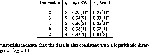
There is little theoretical understanding of why cluster algorithms work so well, and in particular there is no theory which predicts the dynamic critical exponents for a given model. These values can currently only be obtained from measurements using Monte Carlo simulation. Our results, which are the best currently available, are shown in Table 4.6. We would like to know why, for example, critical slowing down is virtually eliminated for the two-dimensional 2-state Potts model, but z is nearly one for the 4-state model; and why the dynamic critical exponents for the SW and Wolff algorithms are approximately the same in two dimensions, but very different in higher dimensions.

Table 4.6: Measured Dynamic Critical Exponents for Potts Model Cluster Algorithms.
The only rigorous analytic result so far obtained for cluster
algorithms was derived by Li and Sokal [Li:89a]. They showed that
the autocorrelation time for the energy using the SW algorithm is
bounded (as a function of the lattice size) by the specific heat  ,
that is,
  , which implies
that the corresponding dynamic critical exponent is bounded by
 , where
  and
and  are critical exponents
measuring the divergence at the critical point of the specific heat and
the correlation length, respectively. A similar bound has also been
derived for the Metropolis algorithm, but with the susceptibility
exponent substituted for the specific heat exponent.
No such result is known for the Wolff algorithm, so we have attempted
to check this result empirically using simulation
[Coddington:92a]. We found that for the Ising model in two, three,
and four dimensions, the above bound appears to be satisfied (at least
to a very good approximation); that is, there are constants a and b
such that  , and thus
 , for the Wolff algorithm.
This led us to investigate similar empirical relations between dynamic
and static quantities for the SW algorithm. The power of cluster
update algorithms comes from the fact that they flip large clusters of
spins at a time. The average size of the largest SW cluster (scaled by
the lattice volume), m, is an estimator of the magnetization for the
Potts model, and the exponent  characterizing the
divergence of the magnetization has values which are similar to our
measured values for the dynamic exponents of the SW algorithm. We
therefore scaled the SW autocorrelations by m, and found that within
the errors of the simulations, this gave either a constant (in three
and four dimensions) or a logarithm (in two dimensions). This implies
that the SW autocorrelations scale in the same way (up to logarithmic
corrections) as the magnetization, that is,
  .
.
These simple empirical relations are very surprising, and if true, would be the first analytic results equating dynamic quantities, which are dependent on the Monte Carlo algorithm used, to static quantities, which depend only on the physical model. These relations could perhaps stem from the fact that the dynamics of cluster algorithms are closely linked to the physical properties of the system, since the Swendsen-Wang clusters are just the Coniglio-Klein-Fisher droplets which have been used to describe the critical behavior of these systems [Fisher:67a] [Coniglio:80a].
We are currently doing further simulations to check whether these relations hold up with larger lattices and better statistics, or whether they are just good approximations. We are also trying to determine whether similar results hold for the general q-state Potts model. However, we have thus far only been able to find simple relations for the q=2 (Ising) model. This work is being done using both parallel machines (the nCUBE-1, nCUBE-2, and Symult S2010) and networks of DEC, IBM, and Hewlett-Packard workstations. These high-performance RISC workstations were especially useful in obtaining good results for the Wolff algorithm, which does not vectorize or parallelize, apart from the trivial parallelism we used in running independent simulations on different processors.


