 -time,
  -memory data
distributions useful for sparse matrix factorizations and the problems that generate
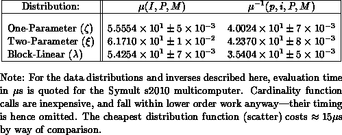
such matrices. We quantify evaluation costs in Table 9.3.


We introduce new closed-form  -time,
  -memory data
distributions useful for sparse matrix factorizations and the problems that generate
such matrices. We quantify evaluation costs in Table 9.3.

Table 9.3: Evaluation Times for Three Data Distributions
Every concurrent data structure is associated with a logical process grid at creation (cf., Figure 9.12 and [Skjellum:90a;90c]). Vectors are either row- or column-distributed within a two-dimensional process grid. Row-distributed vectors are replicated in each process column, and distributed in the process rows. Conversely, column-distributed vectors are replicated in each process row, and distributed in the process columns. Matrices are distributed both in rows and columns, so that a single process owns a subset of matrix rows and columns. This partitioning follows the ideas proposed by Fox et al. [Fox:88a] and others. Within the process grid, coefficients of vectors and matrices are distributed according to one of several data distributions. Data distributions are chosen to compromise between load-balancing requirements and constraints on where information can be calculated in the ensemble.
Definition 1 (Data-Distribution Function)
A data-distribution function
The formal requirements for a data-distribution function are as follows. Let
The cardinality of the set  maps three integers
  where
where  , is the global name of a coefficient, P is
the number of processes among which all coefficients are to be partitioned,
and M is the total number of coefficients. The pair
  represents the
process p (
 ) and local (process-p) name i of the
coefficient (
 ). The inverse distribution
function
  transforms the local name i back
to the global coefficient name I.
 be the set of global coefficient names associated with process
 , defined implicitly by a data distribution function
 . The following set properties must hold:

 , is given by
  .
.
The linear and scatter data-distribution functions are most often defined. We generalize these functions (by blocking and scattering parameters) to incorporate practically important degrees of freedom. These generalized distribution functions yield optimal static load balance as do the unmodified functions described in [Velde:90a] for unit block size, but they differ in coefficient placement. This distinction is technical, but necessary for efficient implementations.
Definition 2 (Generalized Block-Linear)
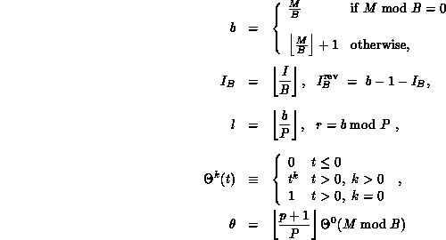
The definitions for the generalized block-linear distribution function,
inverse, and cardinality function are:
while
where B denotes the coefficient block size,
and where
For B=1, a load-balance-equivalent variant of the common linear
data-distribution function is recovered. The general block-linear
distribution function divides coefficients among the P processes


 .
.
 so that each
  is a set of coefficients with
contiguous global names, while optimally load-balancing the b blocks among
the P sets. Coefficient boundaries between processes are on multiples of
B. The maximum possible coefficient imbalance between processes is B.
If
  , the last block in process P-1 will be foreshortened.
Definition 3 (Parametric Functions)
To allow greater freedom in the distribution of coefficients among
processes, we define a new, two-parameter distribution function family,
where
with
and where r, b, etc. are as defined above.
The inverse distribution function
with
For S = 1, a block-scatter distribution results, while for  . The B blocking parameter (just introduced in
the block-linear function) is mainly suited to the clustering of
coefficients that must not be separated by an interprocess boundary
(again, see [Skjellum:90c] for a definition of general
block-scatter,
  ). Increasing B worsens the static load
balance. Adding a second scaling parameter S (of no impact on the
static load balance) allows the distribution to scatter coefficients to
a greater or lesser degree, directly as a function of this one
parameter. The two-parameter distribution function, inverse and
cardinality function are defined below. The one-parameter distribution
function family,
  , occurs as the special case B=1, also as
noted below:


 is defined as
follows:


 , the generalized block-linear distribution
function is recovered. See also [Skjellum:90c].
Definition 4 (Data Distributions)
Given a data-distribution function family
respectively,
A two-dimensional data distribution may be identified as consisting of a row
and column distribution defined over a two-dimensional process grid of
 (
( ), a process list of
P (Q), M (N) as the number of coefficients, and a row (respectively,
column) orientation, a row (column) data distribution
  (
( ) is defined as:


 processes, as
  .
.
Further discussion and detailed comparisons on data-distribution functions are offered in [Skjellum:90c]. Figure 9.13 illustrates the effects of linear and scatter data-distribution functions on a small rectangular array of coefficients.


