

Next: 9.5.3 Reduced-Communication Pivoting
Up: LU Factorization of
Previous: 9.5.1 Introduction
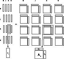
Figure 9.12: Process-Grid Data Distribution of Ax=b. Representation of a
concurrent matrix, and distributed-replicated concurrent vectors on a
 logical process grid. The solution of Ax=b first appears in
x, a column-distributed vector, and then is normally ``transposed'' via a
global combine to the row-distributed vector y.
We solve the problem Ax=b where A is large, and includes many zero
entries. We assume that A is unsymmetric both in sparsity pattern and in
numerical values. In general, the matrix A will be computed in a
distributed fashion, so we will inherit a distribution of the coefficients of
A (cf., Figures 9.12 and 9.13).
Following the style of Harwell's MA28 code for unsymmetric sparse
matrices, we use a two-phase approach to this solution. There is a first LU
factorization called A-mode or ``analyze,'' which builds data structures
dynamically, and employs a user-defined pivoting function. The repeated B-mode
factorization uses the existing data structures statically to factor a new,
similarly structured matrix, with the previous pivoting pattern. B-mode
monitors stability with a simple growth factor estimate. In practice, A-mode
is repeated whenever instability is detected. The two key contributions of
this sparse concurrent solver are reduced communication pivoting, and new
data distributions for better overall performance.
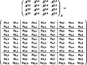
Figure 9.13: Example of Process-Grid Data Distribution. An  array
with block-linear rows (B=2) and scattered columns on a
  logical process grid. Local arrays are denoted at left by
  where
where
 is the grid position of the process on
  . Subscripts
(i.e.,
  ) are the global (I,J) indices.
Following Van de Velde [Velde:90a], we consider the LU factorization of
a real matrix A,  . It is well known (e.g.,
[Golub:89a], pp. 117-118), that for any such matrix A, an LU
factorization of the form

exists, where  are square, (orthogonal) permutation
matrices, and
  are the unit lower- and
upper-triangular factors, respectively. Whereas the pivot sequence is
stored (two N-length integer vectors), the permutation matrices are not
stored or computed with explicitly. Rearranging, based on the orthogonality
of the permutation matrices,
  We factor A with implicit pivoting (no rows or columns are exchanged
explicitly as a result of pivoting). Therefore, we do not store
  directly, but instead:
 . Consequently,
  ,
,  , and
, and
 . The ``unravelling'' of the permutation
matrices is accomplished readily (without implication of additional
interprocess communication) during the triangular solves.
For the sparse case, performance is more difficult to quantify than for
the dense case, but, for example, banded matrices with
bandwidth  can be factored with
  work; we expect subcubic complexity in N for reasonably sparse
matrices, and strive for subquadratic complexity, for very sparse
matrices. The triangular solves can be accomplished in work
proportional to the number of entries in the respective triangular
matrix L or U. The pivoting strategy is treated as a parameter of
the algorithm and is not predetermined. We can consequently treat
the pivoting function as an application-dependent function, and
sometimes tailor it to special problem structures (cf., Section 7 of
[Velde:88a]) for higher performance. As for all sparse
solvers, we also seek subquadratic memory requirements in N,
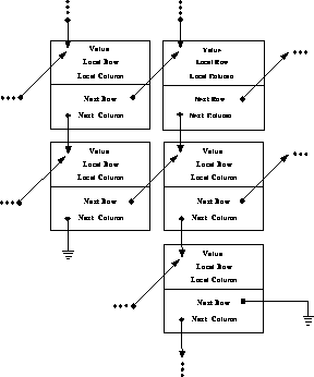
attained by storing matrix entries in linked-list fashion, as
illustrated in Figure 9.14.

Figure 9.14: Linked-list Entry Structure of Sparse Matrix. A single entry
consists of a double-precision value (8 bytes), the local row (i) and column
(j) index (2 bytes each), a ``Next Column Pointer'' indicating the next
current column entry (fixed j), and a ``Next Row Pointer'' indicating the next
current row entry (fixed i), at 4 bytes each. Total: 24 bytes per entry.
For further discussion of LU factorizations and sparse matrices,
see [Golub:89a], [Duff:86a].


Next: 9.5.3 Reduced-Communication Pivoting
Up: LU Factorization of
Previous: 9.5.1 Introduction
Guy Robinson
Wed Mar 1 10:19:35 EST 1995

 logical process grid. The solution of Ax=b first appears in
x, a column-distributed vector, and then is normally ``transposed'' via a
global combine to the row-distributed vector y.


 array
with block-linear rows (B=2) and scattered columns on a
  logical process grid. Local arrays are denoted at left by
  where
where
 is the grid position of the process on
  . Subscripts
(i.e.,
  ) are the global (I,J) indices.
 . It is well known (e.g.,
[
 are square, (orthogonal) permutation
matrices, and
  are the unit lower- and
upper-triangular factors, respectively. Whereas the pivot sequence is
stored (two N-length integer vectors), the permutation matrices are not
stored or computed with explicitly. Rearranging, based on the orthogonality
of the permutation matrices,
  We factor A with implicit pivoting (no rows or columns are exchanged
explicitly as a result of pivoting). Therefore, we do not store
  directly, but instead:
 . Consequently,
  ,
,  , and
, and
 . The ``unravelling'' of the permutation
matrices is accomplished readily (without implication of additional
interprocess communication) during the triangular solves.
 can be factored with
  work; we expect subcubic complexity in N for reasonably sparse
matrices, and strive for subquadratic complexity, for very sparse
matrices. The triangular solves can be accomplished in work
proportional to the number of entries in the respective triangular
matrix L or U. The pivoting strategy is treated as a parameter of
the algorithm and is not predetermined. We can consequently treat
the pivoting function as an application-dependent function, and
sometimes tailor it to special problem structures (cf., Section 7 of
[