


Next: 6.6.5 Comments and Variants
Up: 6.6 Character Recognition by
Previous: 6.6.3 The Multiscale Technique
Here we give some details of our results and compare with the standard
approach. As mentioned in the previous section, a  MLP (1024
inputs, 32 hidden units, 26 output units) was trained on the set of
Figure 6.32 using the multiscale method. Outputs are never
exactly 0 or 1, so we defined a ``successful'' recognition to occur when the
output value of the desired letter was greater than 0.9, and all other
outputs were less than 0.1. The training on the
  grid used
back-propagation with a momentum term and went through the exemplars
sequentially. The weights are changed to reduce the error function for
the current character. The result is that the system does not reach an
absolute minimum. Rather, at long times the weight values oscillate with a
period equal to the time of one sweep through all the exemplars. This is not
a serious problem as the oscillations are very small in practice.
Figure 6.34 shows the training curve for this problem. The first
part of the curve is the training of the
  network; even though the
grid is a bit coarse, almost all of the characters can be memorized.
Proceeding to the next grid by scaling the mesh size by a factor of two and
using the
  exemplars, we obtained the second part of the
learning curve in Figure 6.34. The
  net got 315/320
correct. After 12 additional sweeps on the
  net, a perfect
score of 320/320 is achieved. The third part of Figure 6.34 shows
the result of the final boost to
  . In just two cycles on the
 net, a perfect score of 320/320 was achieved and the training
was stopped. It is useful to compare these results with a direct use of
back-propagation on the
  mesh without using the multiscale
procedure. Figure 6.35 shows the corresponding learning curve,
with the result from Figure 6.34 drawn in for comparison.
Learning via the multiscale method takes much less computer time. In
addition, the internal structure of the resultant network is much different
and we will now turn to this question.
How do these two networks compare for the real task of recognizing exemplars
not belonging to the training set? We used as a generalization test set 156
more handwritten characters. Though there are no ambiguities for humans in
this test set, the networks did make mistakes. The network from the direct
method made errors 14% of the time, and the multiscale network made errors
9% of the time. We feel the improved performance of the multiscale net is
due to the difference in quality of the feature extractors in the two cases.
In a two-layer MLP, we can think of each hidden-layer neuron as a feature
extractor which looks for a certain characteristic shape in the input; the
function of the output layer is then to perform the higher level operation of
classifying the input based on which features it contains. By looking at the
weights connecting a hidden-layer neuron to the inputs, we can determine
what feature that neuron is looking for.
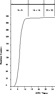
Figure 6.34: The Learning Curve for our Multiscale Training Procedure
Applied to 320 Handwritten Characters. The first part of the curve is
the training on the  net, the second on the
  net, and the last on the full,
  net. The curve is plotted
as a function of CPU time and not sweeps through the presentation set,
in order to exhibit the speed of training on the smaller networks.
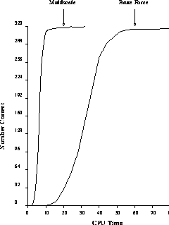
Figure: A Comparison of Multiscale Training with the Usual, Direct
Back-propagation Procedure. The curve labelled ``Multiscale'' is the same as
Figure 6.34, only rescaled by a factor of two. The curve
labelled ``Brute Force'' is from directly training a  network,
from a random start, on the learning set. The direct approach does not quite
learn all of the exemplars, and takes much more CPU time.
For example, Figure 6.36 shows the input weights of two neurons in
the  net. The neuron of (a) seems to be looking for a stroke
extending downward and to the right from the center of the input field. This
is a feature common to letters like A, K, R, and X. The feature extractor of
(b) seems to be a ``NOT S'' recognizer and, among other things, discriminates
between ``S'' and ``Z''.

Figure 6.36: Two Feature Extractors for the Trained  net. This figure
shows the connection weights between one hidden-layer, and all the
input-layer neurons. Black boxes depict positive weights, while white
depict negative weights; the size of the box shows the magnitude. The
position of each weight in the
  grid corresponds to the position
of the input pixel. We can view these pictures as maps of the features which
each hidden-layer neuron is looking for. In (a), the neuron is looking for a
stroke extending down and to the right from the center of the input field;
this neuron fires upon input of the letter ``A,'' for example. In (b), the
neuron is looking for something in the lower center of the picture, but it
also has a strong ``NOT S'' component. Among other things, this neuron
discriminates between an ``S'' and a ``Z''. The outputs of several such
feature extractors are combined by the output layer to classify the original
input.
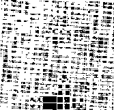
Figure: The Same Feature Extractor as in Figure 6.36(b),
after the Boost to  . There is an obvious correspondence between
each connection in Figure 6.36(b) and
  clumps
of connections here. This is due to the multiscale procedure, and leads to
spatially smooth feature extractors.
Even at the coarsest scale, the feature extractors usually look for blobs
rather than correlating a scattered pattern of pixels. This is encouraging
since it matches the behavior we would expect from a ``good'' character
recognizer. The multiscale process accentuates this locality, since a single
pixel grows to a local clump of four pixels at each rescaling. This effect
can be seen in Figure 6.37, which shows the feature extractor of
Figure 6.36(b) after scaling to  and further
training. Four-pixel clumps are quite obvious in the
  network.
The feature extractors obtained by direct training on large nets are much
more scattered (less smooth) in nature.


Next: 6.6.5 Comments and Variants
Up: 6.6 Character Recognition by
Previous: 6.6.3 The Multiscale Technique
Guy Robinson
Wed Mar 1 10:19:35 EST 1995
 MLP (1024
inputs, 32 hidden units, 26 output units) was trained on the set of
Figure 6.32 using the multiscale method. Outputs are never
exactly 0 or 1, so we defined a ``successful'' recognition to occur when the
output value of the desired letter was greater than 0.9, and all other
outputs were less than 0.1. The training on the
  grid used
back-propagation with a momentum term and went through the exemplars
sequentially. The weights are changed to reduce the error function for
the current character. The result is that the system does not reach an
absolute minimum. Rather, at long times the weight values oscillate with a
period equal to the time of one sweep through all the exemplars. This is not
a serious problem as the oscillations are very small in practice.
Figure 6.34 shows the training curve for this problem. The first
part of the curve is the training of the
  network; even though the
grid is a bit coarse, almost all of the characters can be memorized.
Proceeding to the next grid by scaling the mesh size by a factor of two and
using the
  exemplars, we obtained the second part of the
learning curve in Figure 6.34. The
  net got 315/320
correct. After 12 additional sweeps on the
  net, a perfect
score of 320/320 is achieved. The third part of Figure 6.34 shows
the result of the final boost to
  . In just two cycles on the
 net, a perfect score of 320/320 was achieved and the training
was stopped. It is useful to compare these results with a direct use of
back-propagation on the
  mesh without using the multiscale
procedure. Figure 6.35 shows the corresponding learning curve,
with the result from Figure 6.34 drawn in for comparison.
Learning via the multiscale method takes much less computer time. In
addition, the internal structure of the resultant network is much different
and we will now turn to this question.


 net, the second on the
  net, and the last on the full,
  net. The curve is plotted
as a function of CPU time and not sweeps through the presentation set,
in order to exhibit the speed of training on the smaller networks.
 network,
from a random start, on the learning set. The direct approach does not quite
learn all of the exemplars, and takes much more CPU time.
 net. The neuron of (a) seems to be looking for a stroke
extending downward and to the right from the center of the input field. This
is a feature common to letters like A, K, R, and X. The feature extractor of
(b) seems to be a ``NOT S'' recognizer and, among other things, discriminates
between ``S'' and ``Z''.

 net. This figure
shows the connection weights between one hidden-layer, and all the
input-layer neurons. Black boxes depict positive weights, while white
depict negative weights; the size of the box shows the magnitude. The
position of each weight in the
  grid corresponds to the position
of the input pixel. We can view these pictures as maps of the features which
each hidden-layer neuron is looking for. In (a), the neuron is looking for a
stroke extending down and to the right from the center of the input field;
this neuron fires upon input of the letter ``A,'' for example. In (b), the
neuron is looking for something in the lower center of the picture, but it
also has a strong ``NOT S'' component. Among other things, this neuron
discriminates between an ``S'' and a ``Z''. The outputs of several such
feature extractors are combined by the output layer to classify the original
input.
 . There is an obvious correspondence between
each connection in Figure
  clumps
of connections here. This is due to the multiscale procedure, and leads to
spatially smooth feature extractors.
 and further
training. Four-pixel clumps are quite obvious in the
  network.
The feature extractors obtained by direct training on large nets are much
more scattered (less smooth) in nature.