

Next: 6.6.4 Results
Up: 6.6 Character Recognition by
Previous: 6.6.2 Character Recognition using
We would like to train large, high-resolution nets. If one tries to do this
directly, by simply starting with a very large network and training by the
usual back-propagation methods, not only is the training slow (because of the
large size of the network), but the generalization properties of such nets are
poor. As described above, a large net with many weights from the input layer
to the hidden layer tends to ``grandmother'' the problem, leading to poor
generalization.
The hidden units of an MLP form a set of feature extractors. Considering a
complex pattern such as a Chinese character, it seems clear that some of the
relevant features which distinguish it are large, long-range objects
requiring little detail while other features are fine scale and require high
resolution. Some sort of multiscale decomposition of the problem therefore
suggests itself. The method we will present below builds in long-range
feature extractors by training on small networks and then uses these as an
intelligent starting point on larger, higher resolution networks. The method
is somewhat analogous to the multigrid technique for solving partial
differential equations.
Let us now present our multiscale training algorithm. We begin with the
training set, such as the one shown in Figure 6.32, defined at the
high resolution (in this case,  ). Each exemplar is coarsened by
a factor of two in each direction using a simple grey scale averaging
procedure.
  blocks of pixels in which all four pixels were ``on''
map to an ``on'' pixel, those in which three of the four were ``on'' map to
a ``3/4 on'' pixel, and so on. The result is that each
  exemplar is mapped to a
  exemplar in such a way as to preserve
the large scale features of the pattern. The procedure is then repeated
until a suitably coarse representation of the exemplars is reached. In our
case, we stopped after coarsening to
  .
.
At this point, an MLP is trained to solve the coarse mapping problem by
one's favorite method (back-propagation, simulated annealing, and so on).
In our case, we set up an MLP of 64 inputs (corresponding to  ), 32 hidden units, and 26 output units. This was then trained on
the set of 320 coarsened exemplars using the simple back propagation
method with a momentum term [Rumelhart:86a], Chapter 8.
Satisfactory convergence was achieved after
approximately 50 cycles through the training set.
We now wish to boost back to a high-resolution MLP, using the results of the
coarse net. We use a simple interpolating procedure which works well. We
leave the number of hidden units unchanged. Each weight from the input layer
to the hidden layer is split or ``un-averaged'' into four weights (each now
attached to its own pixel), with each 1/4 the size of the original. The
thresholds are left untouched during this boosting phase. This procedure
gives a higher resolution MLP with an intelligent starting point for
additional training at the finer scale. In fact, before any training at
all is done with the  MLP (boosted from
  ), it recalls
the
  exemplars quite well. This is a measure of how much
information was lost when coarsening from
  to
to  . The
boost and train process is repeated to get to the desired
  MLP.
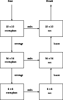
The entire multiscale training process is illustrated in
Figure 6.33.

Figure 6.33: An Example Flowchart for the Multiscale Training Procedure.
This was the procedure used in this text, but the averaging and boosting
can be continued through an indefinite number of stages.


Next: 6.6.4 Results
Up: 6.6 Character Recognition by
Previous: 6.6.2 Character Recognition using
Guy Robinson
Wed Mar 1 10:19:35 EST 1995
 ). Each exemplar is coarsened by
a factor of two in each direction using a simple grey scale averaging
procedure.
  blocks of pixels in which all four pixels were ``on''
map to an ``on'' pixel, those in which three of the four were ``on'' map to
a ``3/4 on'' pixel, and so on. The result is that each
  exemplar is mapped to a
  exemplar in such a way as to preserve
the large scale features of the pattern. The procedure is then repeated
until a suitably coarse representation of the exemplars is reached. In our
case, we stopped after coarsening to
  .
.


 ), 32 hidden units, and 26 output units. This was then trained on
the set of 320 coarsened exemplars using the simple back propagation
method with a momentum term [
 MLP (boosted from
  ), it recalls
the
  exemplars quite well. This is a measure of how much
information was lost when coarsening from
  to
to  . The
boost and train process is repeated to get to the desired
  MLP.
The entire multiscale training process is illustrated in
Figure