Linear Equations


Next: Orthogonal Factorizations and
Up: Computational Routines
Previous: Computational Routines
We use the standard notation for a system of simultaneous
linear
equations :
Ax = b
where A is the coefficient matrix,
b is the right hand side,
and x is the solution.
In (2.4) A is assumed to be a square matrix of order n,
but some of the individual routines allow A to be rectangular.
If there are several right hand sides,
we write
AX = B
where the columns of B are the individual right hand sides,
and the columns of
X are the corresponding solutions.
The basic task is to compute X, given A and B.
If A is upper or lower triangular, (2.4) can be solved by a
straightforward
process of backward or forward substitution.
Otherwise, the solution is obtained after first factorizing A as a
product of
triangular matrices (and possibly also a diagonal matrix or permutation
matrix).
The form of the factorization depends on the properties of the matrix
A.
LAPACK provides routines for the following types of matrices, based on
the stated factorizations:
- general matrices (LU factorization with partial pivoting):
A = PLU
where P is a permutation matrix, L is lower triangular with unit
diagonal elements (lower trapezoidal if m > n), and U is upper
triangular (upper trapezoidal if m < n).
- general band matrices including tridiagonal matrices
(LU factorization with partial pivoting):
If A is m-by-m with kl subdiagonals and ku superdiagonals,
the factorization is
A = LU
where L is a product of permutation and unit lower triangular
matrices with kl subdiagonals, and U is upper triangular with
kl + ku superdiagonals.
- symmetric and Hermitian positive definite matrices including
band matrices (Cholesky factorization):


where U is an upper triangular matrix and L is lower triangular.
- symmetric and Hermitian positive definite tridiagonal matrices (
 factorization):

where U is a unit upper bidiagonal matrix, L is unit lower
bidiagonal, and D is diagonal.
- symmetric and Hermitian indefinite matrices (symmetric indefinite
factorization) :


where U (or L) is a product of permutation and unit upper (lower)
triangular matrices, and D is symmetric and block diagonal with diagonal
blocks of order 1 or 2.
The factorization for a general tridiagonal matrix is like that for
a general band matrix with kl = 1 and ku = 1. The factorization
for a symmetric positive definite band matrix with k superdiagonals
(or
subdiagonals) has the same form as for a symmetric positive definite
matrix, but the factor U (or L) is a band matrix with k
superdiagonals (subdiagonals). Band matrices use a compact band
storage scheme described in section 5.3.3.
LAPACK routines are also provided for symmetric matrices (whether
positive definite or indefinite) using packed storage,
as described in section 5.3.2.
While the primary use of a matrix factorization is to solve a system
of equations, other related tasks are provided as well.
Wherever possible, LAPACK provides routines to perform each of these
tasks
for each type of matrix and storage scheme (see
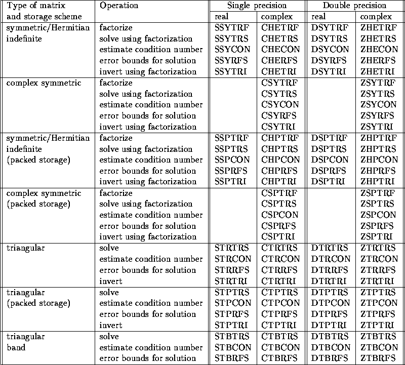
Tables 2.7 and 2.8).
The following list relates the tasks
to the last 3 characters of the name of the corresponding
computational routine:
- xyyTRF:
- factorize (obviously not needed for triangular matrices);
- xyyTRS:
- use the factorization (or the matrix A itself if it is
triangular) to
solve (2.5) by forward or backward substitution;
- xyyCON:
- estimate the reciprocal of the condition number
 ;
Higham's modification [52] of Hager's method [48]
is used to estimate
  ,
except for symmetric positive definite tridiagonal matrices for which it
is computed directly with comparable efficiency [50];
- xyyRFS:
- compute bounds on the error in the computed solution (returned
by the xyyTRS routine), and
refine the solution to reduce the backward error (see below);
- xyyTRI:
- use the factorization (or the matrix A itself if it is
triangular)
to compute
 (not provided for band matrices, because the inverse
does not in general preserve bandedness);
- xyyEQU:
- compute scaling factors to equilibrate A
(not provided for tridiagonal, symmetric
indefinite, or triangular matrices). These routines do not actually scale
the matrices: auxiliary routines xLAQyy may be used for that purpose -
see the code of the driver routines xyySVX for sample usage .
Note that some of the above routines depend on the output of others:
- xyyTRF:
- may work on an equilibrated matrix produced by
xyyEQU and xLAQyy, if yy is one of {GE, GB, PO, PP, PB};
- xyyTRS:
- requires the factorization returned by xyyTRF;
- xyyCON:
- requires the norm of the original matrix A, and the
factorization returned by xyyTRF;
- xyyRFS:
- requires the original matrices A and B, the factorization
returned by xyyTRF, and the solution X returned by xyyTRS;
- xyyTRI:
- requires the factorization returned by xyyTRF.
The RFS (``refine solution'') routines perform iterative
refinement
and compute backward and forward error bounds for the solution.
Iterative refinement is done in the same precision as the input data.
In particular, the residual is not computed with extra precision,
as has been traditionally done.
The benefit of this procedure is discussed in Section 4.4.
--------------------------------------------------------------------------------
Type of matrix     Operation                  Single precision  Double precision
and storage scheme                            real     complex  real     complex
--------------------------------------------------------------------------------
general            factorize                  SGETRF   CGETRF   DGETRF   ZGETRF
                   solve using factorization  SGETRS   CGETRS   DGETRS   ZGETRS
                   estimate condition number  SGECON   CGECON   DGECON   ZGECON
                   error bounds for solution  SGERFS   CGERFS   DGERFS   ZGERFS
                   invert using factorization SGETRI   CGETRI   DGETRI   ZGETRI
                   equilibrate                SGEEQU   CGEEQU   DGEEQU   ZGEEQU
--------------------------------------------------------------------------------
general            factorize                  SGBTRF   CGBTRF   DGBTRF   ZGBTRF
 band              solve using factorization  SGBTRS   CGBTRS   DGBTRS   ZGBTRS
                   estimate condition number  SGBCON   CGBCON   DGBCON   ZGBCON
                   error bounds for solution  SGBRFS   CGBRFS   DGBRFS   ZGBRFS
                   equilibrate                SGBEQU   CGBEQU   DGBEQU   ZGBEQU
--------------------------------------------------------------------------------
general            factorize                  SGTTRF   CGTTRF   DGTTRF   ZGTTRF
 tridiagonal       solve using factorization  SGTTRS   CGTTRS   DGTTRS   ZGTTRS
                   estimate condition number  SGTCON   CGTCON   DGTCON   ZGTCON
                   error bounds for solution  SGTRFS   CGTRFS   DGTRFS   ZGTRFS
--------------------------------------------------------------------------------
symmetric/         factorize                  SPOTRF   CPOTRF   DPOTRF   ZPOTRF
 Hermitian         solve using factorization  SPOTRS   CPOTRS   DPOTRS   ZPOTRS
 positive definite estimate condition number  SPOCON   CPOCON   DPOCON   ZPOCON
                   error bounds for solution  SPORFS   CPORFS   DPORFS   ZPORFS
                   invert using factorization SPOTRI   CPOTRI   DPOTRI   ZPOTRI
                   equilibrate                SPOEQU   CPOEQU   DPOEQU   ZPOEQU
--------------------------------------------------------------------------------
symmetric/         factorize                  SPPTRF   CPPTRF   DPPTRF   ZPPTRF
 Hermitian         solve using factorization  SPPTRS   CPPTRS   DPPTRS   ZPPTRS
 positive definite estimate condition number  SPPCON   CPPCON   DPPCON   ZPPCON
 (packed storage)  error bounds for solution  SPPRFS   CPPRFS   DPPRFS   ZPPRFS
                   invert using factorization SPPTRI   CPPTRI   DPPTRI   ZPPTRI
                   equilibrate                SPPEQU   CPPEQU   DPPEQU   ZPPEQU
--------------------------------------------------------------------------------
symmetric/         factorize                  SPBTRF   CPBTRF   DPBTRF   ZPBTRF
 Hermitian         solve using factorization  SPBTRS   CPBTRS   DPBTRS   ZPBTRS
 positive definite estimate condition number  SPBCON   CPBCON   DPBCON   ZPBCON
 band              error bounds for solution  SPBRFS   CPBRFS   DPBRFS   ZPBRFS
                   equilibrate                SPBEQU   CPBEQU   DPBEQU   ZPBEQU
--------------------------------------------------------------------------------
symmetric/         factorize                  SPTTRF   CPTTRF   DPTTRF   ZPTTRF
 Hermitian         solve using factorization  SPTTRS   CPTTRS   DPTTRS   ZPTTRS
 positive definite estimate condition number  SPTCON   CPTCON   DPTCON   ZPTCON
 tridiagonal       error bounds for solution  SPTRFS   CPTRFS   DPTRFS   ZPTRFS
--------------------------------------------------------------------------------
Table 2.7: Computational routines for linear equations

Table 2.8: Computational routines for linear equations (continued)


Next: Orthogonal Factorizations and
Up: Computational Routines
Previous: Computational Routines
Tue Nov 29 14:03:33 EST 1994


 factorization):


 ;
Higham's modification [52] of Hager's method [48]
is used to estimate
  ,
except for symmetric positive definite tridiagonal matrices for which it
is computed directly with comparable efficiency [50];
 (not provided for band matrices, because the inverse
does not in general preserve bandedness);
