 |
We solved linear systems by GMRES with 30 iteration vectors.
The method was restarted by Morgan's implicitly restarted GMRES [334]
keeping the
15 smallest Ritz pairs in the basis until the residual norm
satisfied
![]() with
with
![]() .
We used Algorithm 11.4 for computing the eigenvalue nearest
.
We used Algorithm 11.4 for computing the eigenvalue nearest
![]() .
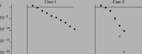
We consider two cases.
For Case 1, we used a fixed
.
We consider two cases.
For Case 1, we used a fixed ![]() .
For Case 2, we used two steps with
.
For Case 2, we used two steps with ![]() and the remaining
steps solved the correction equation (11.5). From the results
in Table 11.2 and Figure 11.1,
we can see linear convergence for
Case 1. Since the linear systems are solved more accurately (
and the remaining
steps solved the correction equation (11.5). From the results
in Table 11.2 and Figure 11.1,
we can see linear convergence for
Case 1. Since the linear systems are solved more accurately (![]() )
than the
speed of the eigenvalue solver,
)
than the
speed of the eigenvalue solver, ![]() and
and ![]() converge to zero with the
same
speed.
For Case 2, the convergence is linear for Steps 1 and 2, since
converge to zero with the
same
speed.
For Case 2, the convergence is linear for Steps 1 and 2, since ![]() is
constant. From the third iteration on,
is
constant. From the third iteration on, ![]() converges quadratically to zero.
The
converges quadratically to zero.
The ![]() converge linearly in steps 1 and 2, then we have quadratic
convergence on steps 3 and 4, and then linear convergence again with
convergence ratio
converge linearly in steps 1 and 2, then we have quadratic
convergence on steps 3 and 4, and then linear convergence again with
convergence ratio ![]() .
.
The residual norm ![]() has two terms.
The first term decreases very rapidly when
has two terms.
The first term decreases very rapidly when ![]() is close to an eigenvalue.
The decrease of the second term (the residual of the linear system solver)
is often much more difficult when the pole lies close to the spectrum.
In practice, we may need to balance the number of outer iterations
(the eigenvalue solver) and the number of inner iterations (the linear
system solver) by selecting the most optimal
is close to an eigenvalue.
The decrease of the second term (the residual of the linear system solver)
is often much more difficult when the pole lies close to the spectrum.
In practice, we may need to balance the number of outer iterations
(the eigenvalue solver) and the number of inner iterations (the linear
system solver) by selecting the most optimal ![]() .
This comment is also related to the end of §11.2.3.
.
This comment is also related to the end of §11.2.3.