

Next: 6.6.2 Character Recognition using
Up: 6.6 Character Recognition by
Previous: 6.6 Character Recognition by
There are many architectures for neural networks; we shall work with
Multi-Layer Perceptrons. These are
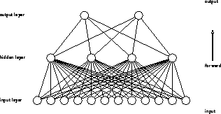
feed-forward networks, and the network to be used in our problem is
schematically shown in Figure 6.31. There are two
processing layers: output and hidden. Each one has a
number of identical units (or ``neurons''), connected in a feed-forward
fashion by wires, often called weights because each one is assigned a
real number  . The input to any given unit is
  ,
where i labels incoming wires and
  is the input (or current) to
that wire. For the hidden layer,
  is the value of a bit of the
input image; for the output layer, it is the output from a unit of
the hidden layer.

Figure 6.31: A Multi-Layer Perceptron
Generally, the output of a unit is a nonlinear, monotonic-increasing
function of the input. We make the usual choice and take

to be our neuron input/output function.  is the threshold and can be
different for each neuron. The weights and thresholds are usually the only
quantities which change during the learning period. We wish to have a
network perform a mapping M from the input space to the output space.
Introducing the actual output
  for an input I, one first chooses a
metric for the output space, and then seeks to minimize
  ,
where d is a measure of the distance between the two points. This quantity
is also called the error function, the energy, or (the negative of) the
harmony function. Naturally,
  depends on the
  's. One can then
apply standard minimization searches like simulated annealing [Kirkpatrick:83a] to attempt to change the
  's so
as to reduce the error. The most commonly used method is gradient
descent, which for MLP is called
back-propagation because the calculation of the
gradients is performed in a feed-backwards fashion. Improved descent
methods may be found in [Dahl:87a], [Parker:87a] and in
Section 9.9 of this book.
The minimization often runs into difficulties because one is searching in a
very high-dimensional space, and the minima may be narrow. In addition,
the straightforward implementation of back-propagation will often fail
because of the many minima in the energy landscape. This process of
minimization is referred to as learning or memorization as the network tries
to match the mapping M. In many problems, though, the input space is so
huge that it is neither conceivable nor desirable to present all possible
inputs to the network for it to memorize. Given part of the mapping M, the
network is expected to guess the rest: This is called generalization. As
shown clearly in [Denker:87a] for the case of a discrete input space,
generalization is often an ill-posed problem: Many generalizations of M
are possible. To achieve the kind of generalization humans want, it is
necessary to tell the network about the mapping one has in mind. This is
most simply done by constraining the weights to have certain symmetries as in
[Denker:87a]. Our approach will be similar, except that the ``outside''
information will play an even more central role during the learning process.


Next: 6.6.2 Character Recognition using
Up: 6.6 Character Recognition by
Previous: 6.6 Character Recognition by
Guy Robinson
Wed Mar 1 10:19:35 EST 1995
 . The input to any given unit is
  ,
where i labels incoming wires and
  is the input (or current) to
that wire. For the hidden layer,
  is the value of a bit of the
input image; for the output layer, it is the output from a unit of
the hidden layer.


 is the threshold and can be
different for each neuron. The weights and thresholds are usually the only
quantities which change during the learning period. We wish to have a
network perform a mapping M from the input space to the output space.
Introducing the actual output
  for an input I, one first chooses a
metric for the output space, and then seeks to minimize
  ,
where d is a measure of the distance between the two points. This quantity
is also called the error function, the energy, or (the negative of) the
harmony function. Naturally,
  depends on the
  's. One can then
apply standard minimization searches like simulated annealing
 's so
as to reduce the error. The most commonly used method is gradient
descent, which for MLP is called
back-propagation