

We obtained many good results which were previously unknown. Among them, the correlation functions are perhaps the most important. First, the results can be directly compared with experiments, thus providing new understanding of the magnetic structure of the high-temperature superconducting materials. Second, and no less important, is the behavior of the correlation function we obtained which gives a crucial test of the assessment of various approximate methods.
In the large spin-S (classical) system, the correlation length goes as

at low temperatures. This predicts a too-large correlation length, compared
with experimental results. As  , the quantum
fluctuations in the system become significant. Several approximate
methods [Chakravarty:88a], [Auerbach:88a] predict a similar low-T
behavior.
  ,
,  , and p=0 or 1.
  is a quantum
renormalization constant.
Our extensive quantum Monte Carlo simulations were performed [Ding:90g]
on the spin- system as large as
  at low
temperature range
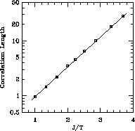
  -1.0. The correlation length, as a
function of
  , is plotted in Figure 6.11. The data points fall
onto a straight line, surprisingly well, throughout the whole temperature
range, leading naturally to the pure exponential form:

where a is the lattice constant. This provides a crucial support to the above-mentioned theories. Quantitatively,

or


Figure 6.11: Correlation Length Measured at Various Temperatures. The
straight line is the fit.
Direct comparison with experiments will not only test the validity of
the Heisenberg model, but also determine the important parameter, the
exchange coupling J. The spacing between Cu atoms in  plane
is
  . Setting
  , the Monte
Carlo data is compared with those from neutron scattering experiments
[Endoh:88a] in Figure 6.5. The agreement is very
good. This provides strong evidence that the essential magnetic
behavior is captured by the Heisenberg model.
The quantum Monte Carlo result is an accurate first
principle calculation; no adjustable parameter is involved. Comparing
directly with the experiment, the only adjustable parameter is J.
This gives an independent determination of the effective exchange
coupling:

Note that near  , the experimentally measured
correlation is systematically smaller than the theoretical curve, shown in
Equation 6.4. This is a combined result of small effects:
frustration, anisotropies, inter-layer coupling, and so on.
Various moments of the Raman spectrum are calculated using series expansions
and comparing with experiments [Singh:89a]. This gives an estimate,
 (
( ), which is quite
close to the above value determined from correlation functions. Raman
scattering probes the short wavelength region, whereas neutron scattering
measures the long-range correlations. The agreement of J's obtained from
these two rather different experiments is another significant indication that
the magnetic interactions are dominated by the Heisenberg model.
Equation 6.4 is valid for all the quantum AFM spins. The classic
two-dimensional antiferromagnetic system discovered twenty years ago
[Birgeneau:71a],  , is a spin-one system with
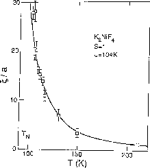
 . Very recently, Birgeneau [Birgeneau:90a] fitted the
measured correlation lengths to

The fit is very good, as shown in Figure 6.12. The factor
( ) comes from integration of the two-loop
  -function without
taking the
  limit, and could be neglected if T is very
close to 0. For the spin-
 AFM
AFM  ,
Equation 6.4 also describes the data quite well [Higgins:88a].

Figure 6.12: Correlation Length of  Measured in Neutron
Scattering Experiment with the Fit.
A common feature from Figures 6.11 and 6.12 is that
the scaling equation Equation 6.4, which is derived near  ,
is valid for a wide range of T, up to
  . This differs
drastically from the range of criticality in three-dimensional systems, where
the width
  is usually about 0.2 or less. This is a
consequence of the crossover temperature
  [Chakravarty:88a],
where the Josephson length scale becomes compatible with the thermal wave
length, being relatively high,
  . This property is a general
character in the low critical dimensions. In the quantum XY model, a
Kosterlitz-Thouless transition occurs
[Ding:90b] at
  and the critical behavior remains valid up
to
  .
.
As emphasized by Birgeneau, the spin-wave value

S=1,  , fits the experiment quite well, whereas for
 , spin-wave value
  differs significantly from the
correct value 1.25 as in Equation 6.4. This indicates that the
large quantum fluctuations in the spin-
 system are not
adequately accounted for in the spin-wave theory, whereas for the spin-one
system, they are.
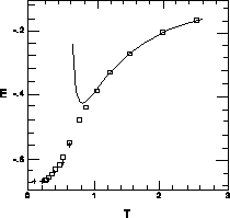
Figure 6.13 shows the energy density at various temperatures. At
higher T, the high-temperature series expansion accurately reproduces our
data. At low T, E approaches a finite ground state energy. Another
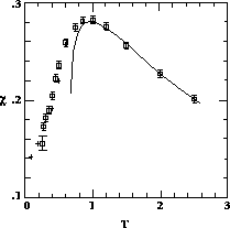
useful thermodynamical quantity is uniform susceptibility, which is shown in
Figure 6.14. Again, at high-T, series expansion coincides with
our data. The maximum point occurs at  with
with
 . This is useful in determining J and
 for the material.

Figure 6.13: Energy Measured as a Function of Temperature. Squares are from
our work. The curve is the 10th order high-T expansion.

Figure: Uniform Susceptibility Measured as a Function of Temperature.
Symbols are similar to Figure 6.13.


