Properties of the Algorithm

While the complex symmetry of $A$ has no effect on the eigenvalues of $A$, this particular structure can be exploited to halve the work and storage requirements of the general non-Hermitian Lanczos method described in §7.8. Indeed, while the non-Hermitian Lanczos method involves one matrix-vector product with $A$ and one with $A^{\ast}$ at each iteration, the complex symmetric Lanczos method only requires one matrix-vector product with $A$ at each iteration.

After $j$ iterations, the complex symmetric Lanczos method has generated $j$ Lanczos vectors,

$$v_1,v_2,\ldots,v_j,$$ (200)

that span the $j$th Krylov subspace ${\cal K}^j(A,b)$ induced by the complex symmetric matrix $A$ and any nonzero starting vector $b$. The vectors (7.94) are constructed to be complex orthogonal:

$$V_j^T V_j = I_j,\quad \mbox{where}\quad V_j = \left[ \begin{array}{cccc} v_1 & v_2 & \cdots & v_j \end{array} \right].$$ (201)

Note that, in view of the eigendecomposition (7.91) of diagonalizable complex symmetric matrices $A$, the complex orthogonality (7.95) of the Lanczos vectors is natural.

The complex symmetric Lanczos algorithm computes the vectors (7.94) by means of three-term recurrences that can be summarized as follows:

$$A V_j = V_j T_j + \left[ \begin{array}{cccc} 0 & \cdots & 0 & \hat{v}_{j+1} \end{array} \right].$$ (202)

Here,

$$T_j = T_j^T = \left[ \begin{array}{cccc} \alpha_1 & \beta_2... ...ots & \beta_j \\ & & \beta_j & \alpha_j \end{array} \right]$$ (203)

is a complex symmetric tridiagonal matrix whose entries are the coefficients of the three-term recurrences. The vector $\hat{v}_{j+1}$ is the candidate for the next Lanczos vector, $v_{j+1}$. It is constructed so that the orthogonality condition

$$V_j^T \hat{v}_{j+1} = 0$$ (204)

is satisfied, and it only remains to be normalized so that $v_{j+1}^T v_{j+1}=1$. However, it cannot be excluded that

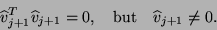$$\hat{v}_{j+1}^T \hat{v}_{j+1} = 0,\quad \mbox{but}\quad \hat{v}_{j+1}\not=0.$$ (205)

If (7.99) occurs, then a next vector $v_{j+1}$ cannot be obtained by simply normalizing $\hat{v}_{j+1}$, as it would require division by zero. Therefore, (7.99) is called a breakdown of the complex symmetric Lanczos algorithm. Breakdowns can be remedied by incorporating look-ahead into the algorithm. Here, for simplicity, we restrict ourselves to the complex symmetric Lanczos algorithm without look-ahead, and we simply stop the algorithm in case a breakdown (7.99) is encountered.

After $j$ iterations of the complex symmetric Lanczos algorithm, approximate eigensolutions for the complex symmetric eigenvalue problem (7.88) are obtained by computing eigensolutions of $T_j$,

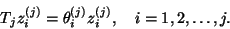$$T_j z_i^{(j)} = \theta_i^{(j)} z_i^{(j)},\quad i=1,2,\ldots,j.$$ (206)

Each value $\theta_i^{(j)}$ and its Ritz vector, $x_i^{(j)} = V_j z_i^{(j)}$, yield an approximate eigenpair of $A$. Note that $T_j$ is the complex orthogonal projection of $A$ onto the space spanned by the Lanczos basis matrix $V_j$, i.e.,

$$T_j = V_j^T A V_j.$$ (207)

Indeed, the relation follows by multiplying (7.96) from the left by $V_j^T$ and by using the orthogonality relations (7.95) and (7.98). Of course, in the complex symmetric Lanczos algorithm, the matrix $T_j$ is not computed via the relation (7.101). Instead, the symmetric tridiagonal structure in the definition (7.97) is exploited and only the diagonal and subdiagonal entries of $T_j$ are explicitly generated.

It should be pointed out that $V_j$ is complex orthogonal, but not unitary, which may have effects for the numerical stability.