Implicit Restart

An unfortunate aspect of the Lanczos or Arnoldi procedure is that there is no way to determine in advance how many steps will be needed to determine the eigenvalues of interest within a specified accuracy. The eigeninformation obtained through this process is completely determined by the choice of the starting vector $v_1$. Unless there is a very fortuitous choice of $v_1$, eigeninformation of interest probably will not appear until $k$ gets very large. Clearly, it becomes intractable to maintain numerical orthogonality of $V_k$. Extensive storage will be required, and repeatedly finding the eigensystem of $H_k$ also becomes expensive at a cost of $O(k^3)$ floating point operations.

The obvious need to control this cost has motivated the development of restarting schemes. Restarting means replacing the starting vector $v_1$ with an ``improved" starting vector $v_1^+$ and then computing a new Arnoldi factorization with the new vector. The structure of $f_k$ serves as a guide: Our goal is to iteratively force $v_1$ to be a linear combination of eigenvectors of interest. In theory, $f_k$ will vanish if $v_1$ is a nontrivial linear combination of $k$ eigenvectors of $A$. However, a more general and, in fact, a better numerical strategy, is to force the starting vector to be a linear combination of Schur vectors that span the desired invariant subspace.

The need for restarting was recognized early on by Karush [258] soon after the appearance of the original algorithm of Lanczos  [285]. Subsequently, there were developments by Paige [347], Cullum and Donath [89], and Golub and Underwood [197]. More recently, a restarting scheme for eigenvalue computation was proposed by Saad based upon the polynomial acceleration scheme originally introduced by Manteuffel [316] for the iterative solution of linear systems. All of these schemes are explicit in the sense that a new starting vector is produced by some process, and then an entirely new Arnoldi factorization is constructed.

There is another approach to restarting that offers a more efficient and numerically stable formulation. This approach, called implicit restarting, is a technique for combining the implicitly shifted QR scheme with a $k$-step Arnoldi or Lanczos factorization to obtain a truncated form of the implicitly shifted QR iteration. The numerical difficulties and storage problems normally associated with Arnoldi and Lanczos procedures are avoided. The algorithm is capable of computing a few ($k$) eigenvalues with user-specified features such as largest real part or largest magnitude using $2nk + O(k^2)$ storage. The computed Schur basis vectors for the desired $k$-dimensional eigenspace are numerically orthogonal to working precision.

Implicit restarting provides a means to extract interesting information from large Krylov subspaces while avoiding the storage and numerical difficulties associated with the standard approach. It does this by continually compressing the interesting information into a fixed-size $k$-dimensional subspace. This is accomplished through the implicitly shifted QR mechanism. An Arnoldi factorization of length $m = k+p$, A V_m = V_m H_m + f_m e_m^ , is compressed to a factorization of length $k$ that retains the eigeninformation of interest. This is accomplished using QR steps to apply $p$ shifts implicitly. The first stage of this shift process results in A V_m^+ = V_m^+ H_m^+ + f_m e_m^ Q , where $V_m^+ = V_m Q$, $H_m^+ = Q^{\ast} H_m Q$, and $Q = Q_1Q_2 \cdots Q_p.$ Each $Q_j$ is the orthogonal matrix associated with the shift $\mu_j$ used during the shifted QR algorithm. Because of the Hessenberg structure of the matrices $Q_j$, it turns out that the first $k-1$ entries of the vector $e_m^{\ast} Q$ are zero. This implies that the leading $k$ columns in equation (7.13) remain in an Arnoldi relation. Equating the first $k$ columns on both sides of (7.13) provides an updated $k$-step Arnoldi factorization A V_k^+ = V_k^+ H_k^+ + f_k^+ e_k^ , with an updated residual of the form $f_k^+ = V_m^+ e_{k+1} \hbeta_k + f_m \sigma$. Using this as a starting point it is possible to apply $p$ additional steps of the Arnoldi procedure to return to the original $m$-step form.

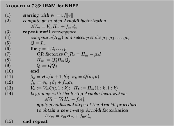
A template for computing a $k$-step Arnoldi factorization with implicit restart is given in Algorithm 7.7.

We will now describe some implementation details, referring to the respective phases in Algorithm 7.7.

(1)

Choose the initial starting vector $v$, normalize and compute an initial $(m = k+p)$-step Arnoldi factorization. Ideally, for eigenvalue calculations, one should attempt to construct a $v$ that is dominant in eigenvector directions of interest. If there is a sequence of closely related eigenvalue problems, this vector should be taken as a linear combination of the eigenvectors (or Schur vectors) of interest from the previous problem. In the absence of any other considerations, a random vector is a reasonable choice.

(3)

A Ritz pair $(x, \theta)$ is ``converged" if $\Vert f_k\Vert\vert e_k^*y\vert<\Vert H_k\Vert\epsilon_D$ where $x = V_k y$ and $\theta$ is ``wanted.'' Upon convergence, this pair should be deflated. See the discussion of deflation in §7.6.6.

(4)

Shift selection: The shifts $\mu_j$ are selected with respect to the user's ``wanted set" specification and the current and perhaps past information about the spectrum of $H_m$. A successful strategy has been to sort the eigenvalues of $H_m$ into a ``wanted set" $\theta_1, \theta_2, \ldots, \theta_k$ and an ``unwanted set" $\mu_1, \mu_2, \ldots, \mu_p$ and take the latter as the selected set of shifts. This is called the exact shift strategy. Other strategies are discussed below.

Examples of the ``wanted set" specification are

the $k$ eigenvalues with largest real part,

the $k$ eigenvalues with largest magnitude,

the $k$ eigenvalues with smallest real part,

the $k$ eigenvalues with smallest magnitude.

(6)-(10)

Apply $p$ steps of the shifted QR iteration to $H_m$ using the $\mu_1, \mu_2, \ldots, \mu_p$ as shifts. This should be done using the implicitly shifted QR variant. If exact shifts are used, then $\beta_{k} = H_m(k+1,k)$ should be zero on completion of the $p$ steps of QR, and the leading submatrix $H_m(1:k,1:k)$ should have $\theta_1, \theta_2, \ldots, \theta_k$ as its eigenvalues.

(12)

When exact shifts are used, then the properties mentioned in (6)-(10) are usually approximately true in finite precision. However, they might not be achieved due to rounding errors. Therefore, it is important to include both terms in the update of the residual vector $f_k \leftarrow v_{k+1}\beta_{k} + f_m \sigma_k$, even though the term $v_{k+1}\beta_{k}$ should be zero in exact arithmetic. Note, with exact shifts, the updated $V_k$ and $H_k$ will provide a new $k$-step Arnoldi factorization with Ritz values and vectors that are the best approximations to the user specification that have been produced so far.

(14)

This step requires a slight modification of the Arnoldi factorization discussed previously. It simply begins with step $k$ of the usual scheme.

There are many ways to select the shifts $\{ \mu_j \}$ that are applied by the QR steps. Virtually any explicit polynomial restarting scheme could be applied through this implicit mechanism. Considerable success has been obtained with the choice of exact shifts. This selection is made by sorting the eigenvalues of $H_m$ into two disjoint sets of $k$ ``wanted" and $p$ ``unwanted" eigenvalues and using the $p$ unwanted ones as shifts. With this selection, the $p$ shift applications result in $H_k^+$ having the $k$ wanted eigenvalues as its spectrum.

Other interesting strategies include the roots of Chebyshev polynomials [383], harmonic Ritz values [331,337,349,411], the roots of Leja polynomials [23], the roots of least squares polynomials [384], and refined shifts [244]. In particular, the Leja and harmonic Ritz values have been used to estimate the interior eigenvalues of $A$.