In this chapter we consider the singular value decomposition (SVD)
of the ![]() by
by ![]() matrix
matrix ![]() . We assume without loss of generality
that
. We assume without loss of generality
that ![]() ; if
; if ![]() consider
consider ![]() .
As described in §2.4, this decomposition
may be written
.
As described in §2.4, this decomposition
may be written
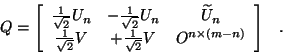
![]() may also be written
may also be written ![]() or
or
![]() for
for ![]() .
.
![]() may also be written
may also be written
![]() or
or
![]() for
for ![]() and
and ![]() for
for
![]() .
.
There are several ``smaller'' versions of the SVD that are
often computed.
Let
![]() be an
be an ![]() by
by ![]() matrix
of the first
matrix
of the first ![]() left singular vectors,
left singular vectors,
![]() be an
be an ![]() by
by ![]() matrix
of the first
matrix
of the first ![]() right singular vectors,
and
right singular vectors,
and
![]() be a
be a
![]() by
by ![]() matrix of the first
matrix of the first ![]() singular values.
Then we have the following SVD types.
singular values.
Then we have the following SVD types.
The thin SVD may also be written
![]() .
Each
.
Each
![]() is called a singular triplet.
The compact and truncated SVDs may be written similarly
(the sum going from
is called a singular triplet.
The compact and truncated SVDs may be written similarly
(the sum going from ![]() to
to ![]() , or
, or ![]() to
to ![]() , respectively).
, respectively).
The SVD of ![]() is closely related to the eigendecompositions of
three related Hermitian matrices,
is closely related to the eigendecompositions of
three related Hermitian matrices, ![]() ,
, ![]() , and
, and
![]() ,
which were described in §2.4.7.
Most iterative algorithms for the SVD amount to applying an algorithm
from Chapter 4
to one of these Hermitian matrices, so we review and expand
that material here.
The choice of
,
which were described in §2.4.7.
Most iterative algorithms for the SVD amount to applying an algorithm
from Chapter 4
to one of these Hermitian matrices, so we review and expand
that material here.
The choice of ![]() ,
, ![]() , or
, or ![]() depends on which singular
values and vectors one is interested in computing.
The cost of some algorithms, like shift-and-invert (see below),
may different significantly for
depends on which singular
values and vectors one is interested in computing.
The cost of some algorithms, like shift-and-invert (see below),
may different significantly for ![]() ,
, ![]() , and
, and ![]() .
.
Thus, if we find the eigenvalues ![]() and eigenvectors
and eigenvectors ![]() of
of ![]() , then we can recover the compact SVD of
, then we can recover the compact SVD of ![]() by taking
by taking
![]() for
for ![]() ,
the right singular vectors as
,
the right singular vectors as ![]() for
for ![]() ,
and the first
,
and the first ![]() left singular vectors by
left singular vectors by
![]() .
The left singular vectors
.
The left singular vectors
![]() through
through ![]() are not determined directly, but may be taken
as any
are not determined directly, but may be taken
as any ![]() orthonormal vectors also orthogonal to
orthonormal vectors also orthogonal to ![]() through
through ![]() .
When
.
When
![]() is very small, i.e.,
is very small, i.e.,
![]() ,
then
,
then ![]() will not be determined very accurately.
will not be determined very accurately.
Thus, if we find the eigenvalues ![]() and eigenvectors
and eigenvectors ![]() of
of ![]() , then we can recover the compact SVD of
, then we can recover the compact SVD of ![]() by taking
by taking
![]() for
for ![]() , the left singular vectors
as
, the left singular vectors
as ![]() for
for ![]() , and the
first
, and the
first ![]() right singular vectors as
right singular vectors as
![]() .
The right singular vectors
.
The right singular vectors ![]() through
through ![]() are
not determined directly, but may be taken as any
are
not determined directly, but may be taken as any ![]() orthonormal
vectors also orthogonal to
orthonormal
vectors also orthogonal to ![]() through
through ![]() .
When
.
When
![]() is very small, i.e.,
is very small, i.e.,
![]() ,
then
,
then ![]() will not be determined very accurately.
will not be determined very accurately.
We note that
The correspondence between the SVD of ![]() and the eigendecomposition
of
and the eigendecomposition
of ![]() shows that the discussion of perturbation theory for
eigenvalues and eigenvectors of Hermitian matrices in
§4.1 and
§4.8 applies directly to the SVD, as we now describe.
shows that the discussion of perturbation theory for
eigenvalues and eigenvectors of Hermitian matrices in
§4.1 and
§4.8 applies directly to the SVD, as we now describe.
Perturbing ![]() to
to ![]() can change the singular values by
at most
can change the singular values by
at most ![]() :
:
Now suppose
![]() is an approximation
of the singular triplet
is an approximation
of the singular triplet
![]() , where
, where
![]() and
and ![]() are unit vectors. The ``best''
are unit vectors. The ``best'' ![]() corresponding to
corresponding to ![]() and
and ![]() is the Rayleigh quotient
is the Rayleigh quotient
![]() , so we assume that
, so we assume that
![]() has this value. Suppose
has this value. Suppose ![]() is closer
to
is closer
to ![]() than any other
than any other ![]() , and let
, and let ![]() be the
gap
between
be the
gap
between ![]() and any other singular value:
and any other singular value:
![]() .
.
The difference between ![]() and
and ![]() is
bounded by
is
bounded by
![]() is easy to compute given
is easy to compute given ![]() ,
, ![]() , and
, and ![]() ,
but
,
but ![]() requires more information about the singular values
in order to approximate it. Typically one uses the computed
singular values near
requires more information about the singular values
in order to approximate it. Typically one uses the computed
singular values near ![]() to approximate
to approximate ![]() :
:
![]() ,
where
,
where
![]() is the next computed singular value smaller than
is the next computed singular value smaller than
![]() , and
, and
![]() is the next computed
singular value larger than
is the next computed
singular value larger than ![]() .
.