 points. The variables
At first it may appear that the sequential time of solving a
factorization is of the order of the number of variables, but things
are not quite that bad. Consider the special case of central
differences on a regular domain of  points. The variables

Figure: Wavefront solution of  from a central difference problem
on a domain of
  points.
on any diagonal in the domain, that is,
in locations  with
with  , depend
only on those on the previous diagonal, that is, with
  .
Therefore it is possible to process the operations on such a diagonal,
or `wavefront' ,
in parallel (see figure
 ![]() ),
or have a vector computer pipeline them;
see Van der Vorst [205][203].
),
or have a vector computer pipeline them;
see Van der Vorst [205][203].
Another way of vectorizing the solution of the triangular factors is
to use some form of expansion of the inverses of the factors.
Consider for a moment a lower triangular matrix, normalized to
the form  where
where  is strictly lower triangular). Its
inverse can be given as either of the following two series:
(The first series is called a ``Neumann expansion'', the second an ``Euler expansion''. Both series are finite, but their length prohibits practical use of this fact.) Parallel or vectorizable preconditioners can be derived from an incomplete factorization by taking a small number of terms in either series. Experiments indicate that a small number of terms, while giving high execution rates, yields almost the full precision of the more recursive triangular solution (see Axelsson and Eijkhout [15] and Van der Vorst [201]).
There are some practical considerations in implementing these
expansion algorithms. For instance, because of the normalization the
 in equation (
![]() ) is not
) is not  . Rather, if we
have a preconditioner (as described in section
 ![]() )
described by
)
described by

then we write

Now we can choose whether or not to store the product  .
Doing so doubles the storage requirements for the matrix, not doing so
means that separate multiplications by
  and
and  have to be
performed in the expansion.

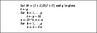
Figure: Preconditioning step algorithm for
a Neumann expansion  of an incomplete factorization
  .
.
Suppose then that the products  and
and  have been
stored. We then define
  by
by
and replace solving a system  for
for  by computing
  .
This algorithm is given in figure
 ![]() .
.