

Next: 13.2.4 Mapping Data to
Up: A Software Tool
Previous: 13.2.2 Overview of the
Given a sequential Fortran program and a selected program segment
(which in the preliminary version can only be a loop nest), the tool
provides assistance in deriving a set of reasonable data partitions for
the arrays accessed in that segment. The assistance is given in the
form of data dependence information for variables accessed within the
selected segment. When partitioning data, we must ensure that the
parallel computations done by all the processors on their local
partitions preserve the data dependence relations in the sequential
program segment. If the computations done by the processors on the
distributed data satisfy all the data dependences, the results of the
computation will be the same as those produced by a sequential
execution of the original program segment. There are two ways to
achieve this: (1) by ``internalizing'' data dependences within each
partition, so that all values required by computations local to a
processor are available in its local data subdomain; or (2) by
inserting appropriate communication to get the nonlocal data.
Let us consider a sample program segment and see how data dependence
information can be used to help derive reasonable data partitionings
for the arrays accessed in the segment.
 MMMMMMMMMMMMMMMMMMMMMMMMMM¯P1. Example program segment.

 *
do j = 1, n

		 do i = 1, n

				 A(i, j) = ( A(i-1, j) )

				 B(i, j) = ( A(i, j), B(i, j-1), B(i, j) )

		 enddo

enddo
 and
and  represent arbitrary functions, and their exact
nature is irrelevant to this discussion. When the programmer selects the
``do i'' loop, the tool indicates that there is one data dependence
that is carried by the i loop: the dependence of
  on
on
 . This dependence indicates that the computation of
an element of A cannot be started until the element immediately above
it in the previous row has been computed. The programmer then selects the
outer ``do j'' loop to get the data dependences that are carried by the
j loop. There is one such dependence, that of
  on
on
 . This dependence indicates that the computation of an
element of B cannot be started until the computation of the element
immediately to the left of it in the previous column has been computed.
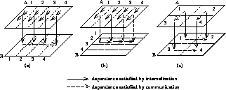
Figure 13.7(a) illustrates the pattern of data dependences for the
above program segment.

Figure 13.7: Data Dependences Satisfied by Internalization and Communication
for the Partitioning Schemes (a) A by Column, B by Column (b) A by Column,
B by Row and (c) A by Block, B by Block. Dotted lines represent partition
boundaries and numbers indicate virtual processor ids (the figures are shown
for p = 4 virtual processors). For clarity, only a few of the dependences
are shown.
The pattern of data dependences between references to elements of an array
gives the programmer clues about how to partition the array. It is usually a
good strategy to partition an array in a manner that internalizes all data
dependences within each partition, so that there is no need to move data
between the different partitions that are stored on different processors.
This avoids expensive communication via messages. For example, the data
dependence of  on
on  can be satisfied by
partitioning A in a columnwise manner, so that the dependences are
``internalized'' within each partition. The data dependence of
 on
on  can be satisfied by partitioning B
row-wise, since this would internalize the dependences within each partition.
It is not enough to examine only the dependences that arise due to
references to the same array. In some cases, the data flow in the program
implicitly couples two different arrays together, so that the partitioning
of one affects the partitioning of the other. In our example, each point
 also requires the value
  . We treat this as a
special data dependence (3) called a value dependence (read ``B is
value dependent on A''), to distinguish it from the traditional data
dependence that is defined only between references to the same array. This
value dependence must also be satisfied either by internalization or by
communication. Internalization of the value dependence is possible only by
partitioning B in the same manner as A, so that each
  and
the
  value required by it are in the same partition.
Based on the pattern of data dependences in the program segment, the
following are a possible list of partitioning choices that can be
derived:\
-
Partition A by column and B by column. This satisfies the dependences within
A and the value dependences of B on A by internalization but communication is
required to satisfy the data dependences within B (Figure 13.7(a)).
An analogous case is to partition both A and B by row. This would require
communication to satisfy dependences within A.
-
Partition A by column and B by row. Dependences within B are now satisfied by
internalization, but communication is needed to satisfy the value dependence
of B on A (Figure 13.7(b)).
-
Partition both A and B as two-dimensional blocks. This would result in
communication to satisfy dependences within both A and B, while the value
dependence of B on A is satisfied by internalization
(Figure 13.7(c)).
The partitioning of A by row and B by column was not considered among the
possible choices because, in this scheme, none of the dependences are
internalized, thus requiring greater communication compared to (1), (2) or
(3). Communication overhead is a major cause of performance degradation
on most machines, so a reasonable first choice would be the partitioning
scheme that requires the least communication. This can be determined either
by analyzing the number of dependences that are cut by the partitioning
(indicating the need for communication), or more accurately using the
performance estimation module that is described in the next section.


Next: 13.2.4 Mapping Data to
Up: A Software Tool
Previous: 13.2.2 Overview of the
Guy Robinson
Wed Mar 1 10:19:35 EST 1995
( A(i-1, j) )
( A(i, j), B(i, j-1), B(i, j) )
 and
and  represent arbitrary functions, and their exact
nature is irrelevant to this discussion. When the programmer selects the
``do i'' loop, the tool indicates that there is one data dependence
that is carried by the i loop: the dependence of
  on
on
 . This dependence indicates that the computation of
an element of A cannot be started until the element immediately above
it in the previous row has been computed. The programmer then selects the
outer ``do j'' loop to get the data dependences that are carried by the
j loop. There is one such dependence, that of
  on
on
 . This dependence indicates that the computation of an
element of B cannot be started until the computation of the element
immediately to the left of it in the previous column has been computed.
Figure 13.7(a) illustrates the pattern of data dependences for the
above program segment.


 on
on  can be satisfied by
partitioning A in a columnwise manner, so that the dependences are
``internalized'' within each partition. The data dependence of
 on
on  can be satisfied by partitioning B
row-wise, since this would internalize the dependences within each partition.
 also requires the value
  . We treat this as a
special data dependence (3) called a value dependence (read ``B is
value dependent on A''), to distinguish it from the traditional data
dependence that is defined only between references to the same array. This
value dependence must also be satisfied either by internalization or by
communication. Internalization of the value dependence is possible only by
partitioning B in the same manner as A, so that each
  and
the
  value required by it are in the same partition.