

Next: 12.4.4 Acquiring Locally Essential
Up: 12.4 Tree Codes for
Previous: 12.4.2 Computing Forces
Computational science advances both in hardware and algorithms.
Occasionally, algorithmic advances are of such tremendous significance that
they completely overshadow the striking advances constantly being made by
hardware. Tree codes are just such an algorithmic advance. It is literally
true that a tree code running on a modest workstation can address larger
problems than can the fastest parallel supercomputer running an  algorithm. It is well known [Fox:84e], [Fox:88a] that parallel
computers can efficiently evaluate the
  force evaluations required by
direct application of Equation 12.5. However, this fact is of
limited significance now that a new class of algorithms has changed the
underlying complexity of the problem. If parallel computers are to have an
impact on the N-body problem, then they must be able to efficiently execute
tree codes.
Parallelization of tree codes is a challenging problem. Typical
astrophysical simulations are highly inhomogeneous. Spatial densities can
vary by a factor of  or more through the computational domain. The
tree must be adaptive to deal with such a large dynamic range in densities,
that is, it must be deep in regions of high particle density, and shallow in
regions of low particle density. Furthermore, the structure of the
inhomogeneities is often dynamic-for example, galaxies form, move, collide, and
merge in cosmological simulations. A fixed tree and/or a fixed decomposition
is not suitable for such a system. Despite these problems, it is possible to
find parallelism in tree codes and to run them efficiently on large parallel
computers [Fox:89t], [Salmon:90a], [Warren:92a;93a].
The technique of ``domain decomposition'' has been applied with excellent
results to a number of other problem areas. We have found that a slightly
abstracted concept of domain decomposition is also applicable to tree codes.
Recall that a domain decomposition usually proceeds by ``assigning'' spatial
domains to processors. In designing a parallel program, the precise meaning
of ``assign'' is crucial. We adopt the following ``owner-computes''
definition of a domain: A domain is a rectangular region of simulation
space. Assignment of a domain to a processor implies that the processor will
be responsible for updating the positions and velocities of all particles
located within that region of simulation space. We allow that processor
domains might change from one time step to the next, based, presumably, on
load-balancing considerations.
Processor domains are chosen using orthogonal recursive
bisection, or ORB (see
Section 11.1.5). Recall that ORB tries repeatedly to split
some measure of the ``load'' in half, and assign the halves to sets of
processors. In the present context, that means finding a coordinate so
that half of the computational ``load'' is associated with particles
above the split, and half is associated with particles below the
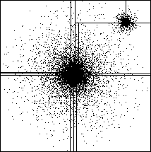
split. The result of applying orthogonal recursive bisection to a
system containing two ``galaxies,'' (well-separated regions with high
local particle density) is shown in Figure 12.13.

Figure 12.13: Decomposition Resulting from Orthogonal Recursive
Bisection of a System with Two Galaxies
It is a simple matter to record the ``load'' associated with each particle.
For example, one can count interactions, or one could simply read the clock
before and after the force on the particle is computed. Then, in order to
find the splitting coordinate, one simply executes a binary (or more
sophisticated) search, seeking a value of the coordinate for which half of
the per-particle work is above and half is below.
In fact, seeking the exact median coordinate of the per-particle work does
not necessarily guarantee load balance. It
guarantees load balance within the force calculation, but it
does not account for load imbalance that may result during construction
of the tree, or during the other phases of the computation. It is
possible to account for these sources of load imbalance by seeking a
coordinate which is not precisely at the median (i.e.,  percentile), but rather at another percentile. The new target
percentile is found by measuring the actual load imbalance, and
adjusting the target by a small amount on each time step to reduce the
observed load imbalance [Salmon:90a].


Next: 12.4.4 Acquiring Locally Essential
Up: 12.4 Tree Codes for
Previous: 12.4.2 Computing Forces
Guy Robinson
Wed Mar 1 10:19:35 EST 1995
 algorithm. It is well known [Fox:84e], [Fox:88a] that parallel
computers can efficiently evaluate the
  force evaluations required by
direct application of Equation 12.5. However, this fact is of
limited significance now that a new class of algorithms has changed the
underlying complexity of the problem. If parallel computers are to have an
impact on the N-body problem, then they must be able to efficiently execute
tree codes.


 or more through the computational domain. The
tree must be adaptive to deal with such a large dynamic range in densities,
that is, it must be deep in regions of high particle density, and shallow in
regions of low particle density. Furthermore, the structure of the
inhomogeneities is often dynamic-for example, galaxies form, move, collide, and
merge in cosmological simulations. A fixed tree and/or a fixed decomposition
is not suitable for such a system. Despite these problems, it is possible to
find parallelism in tree codes and to run them efficiently on large parallel
computers [
 percentile), but rather at another percentile. The new target
percentile is found by measuring the actual load imbalance, and
adjusting the target by a small amount on each time step to reduce the
observed load imbalance [