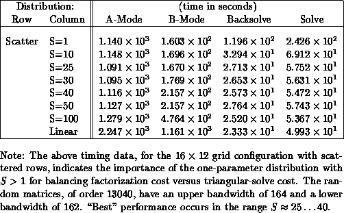
Table 9.4: Order 13040 Band Matrix Performance


Table 9.4: Order 13040 Band Matrix Performance
We consider an order 13040 banded matrix with a
bandwidth of 326 under partial row pivoting. For this
example, we have compiled timing results for a  process
grid with random matrices (entries have range 0-10,000), using
different values of S on the column distribution
(Table 9.4). We indicate timing for A-mode, B-mode,
Backsolves and Forward- and Backsolves together (``Solve'' heading).
For this example, S=30 saves
  of the triangular solve cost
compared to S=1, or approximately 186 seconds, roughly 6 seconds
above the linear optimal. Simultaneously, we incur about 17 seconds
additional cost in B-mode, while saving about 93 seconds in the
Backsolve. Assuming
 , in the first
above-mentioned objective function, we save about 262 (respectively,
76) seconds. Based on this example, and other experiences, we conclude
that this is a successful practical technique for improving overall
sparse linear algebra performance. The following example further
bolsters this conclusion.