Let us first discuss how to distribute
a narrow band matrix A
over a one-dimensional process grid
using a block-column distribution.
We assume that the coefficient band
matrix A
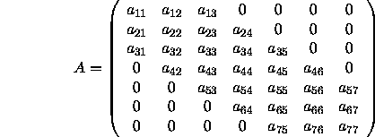
is of size ![]() (
(![]() )
with a bandwidth BW=2 if the matrix
A is symmetric positive definite,
and BWL=2 and BWU=2 if the matrix
A is nonsymmetric. The matrix A is
represented by the following.
)
with a bandwidth BW=2 if the matrix
A is symmetric positive definite,
and BWL=2 and BWU=2 if the matrix
A is nonsymmetric. The matrix A is
represented by the following.
If we assume that the matrix A
is nonsymmetric band, the user may
choose to perform partial pivoting
or no pivoting during the factorization
(PxGBTRF
or PxDBTRF ,
respectively). Both strategies
assume a block-column distribution
of the coefficient matrix, but
additional storage is required
for fill-in if partial pivoting
is selected. First, let us assume
that we have selected no pivoting,
and we distribute this matrix onto
a ![]() process grid with a
block size of
process grid with a
block size of ![]() . The
processes would contain the local
arrays found in figure 4.9.
Figure 4.9
also illustrates that the leading
dimension of the local arrays
containing the coefficient matrix
must be at least BWL+1+BWU for
the non-pivoting narrow band linear
solver.
. The
processes would contain the local
arrays found in figure 4.9.
Figure 4.9
also illustrates that the leading
dimension of the local arrays
containing the coefficient matrix
must be at least BWL+1+BWU for
the non-pivoting narrow band linear
solver.
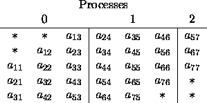
Figure 4.9: Mapping of local arrays for nonsymmetric band matrix A
(no pivoting)
If, however, we select partial pivoting
and distribute this same matrix onto a
![]() process grid with a block
size of
process grid with a block
size of ![]() , the processes would
contain the local arrays found in
figure 4.10.
The amount of additional storage
required for fill-in is represented
by F in the figure and is equal
to the sum of the lower bandwidth
(number of subdiagonals), BWL, and
the upper bandwidth (number of
superdiagonals), BWU. In this
example, BWL=2 and BWU=2.
Refer to the leading comments
of the routine PxGBTRF for
further details. Figure 4.10
also illustrates that the leading
dimension of the local arrays
containing the coefficient matrix
must be at least 2*(BWL+BWU)+1
for the partial pivoting narrow
band linear solver.
, the processes would
contain the local arrays found in
figure 4.10.
The amount of additional storage
required for fill-in is represented
by F in the figure and is equal
to the sum of the lower bandwidth
(number of subdiagonals), BWL, and
the upper bandwidth (number of
superdiagonals), BWU. In this
example, BWL=2 and BWU=2.
Refer to the leading comments
of the routine PxGBTRF for
further details. Figure 4.10
also illustrates that the leading
dimension of the local arrays
containing the coefficient matrix
must be at least 2*(BWL+BWU)+1
for the partial pivoting narrow
band linear solver.
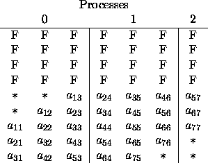
Figure 4.10: Mapping of local arrays for nonsymmetric band matrix
A (partial pivoting)
Let us now assume that the matrix A is
symmetric positive definite band with BW=2,
and we distribute this matrix assuming lower
triangular storage (UPLO='L') onto a ![]() process grid with a block size
process grid with a block size ![]() .
The processes would contain the local arrays
found in figure 4.11. We would
then call the routine
PxPBTRF
with BW=2 to perform the factorization,
for example.
.
The processes would contain the local arrays
found in figure 4.11. We would
then call the routine
PxPBTRF
with BW=2 to perform the factorization,
for example.
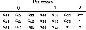
Figure 4.11: Mapping of local arrays for symmetric positive definite
band matrix A (UPLO='L')
If we then distributed this same matrix assuming
upper triangular storage (UPLO='U') onto a ![]() process grid with a block size
process grid with a block size ![]() , the processes
would contain the local arrays found in figure 4.12.
, the processes
would contain the local arrays found in figure 4.12.
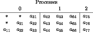
Figure 4.12: Mapping of local arrays for symmetric positive definite
band matrix A (UPLO='U')
Figures 4.11 and 4.12 also illustrate that the leading dimension of the local arrays containing the coefficient matrix must be at least BW+1 for the symmetric positive definite narrow band linear solver.
The ![]() notation in
figures 4.9,
4.10, 4.11,
and 4.12 and the
F notation in figure 4.10
signify an entry in which one
need not store a value in that
position of the local array.
These storage positions, however,
are required and overwritten
during the computation.
notation in
figures 4.9,
4.10, 4.11,
and 4.12 and the
F notation in figure 4.10
signify an entry in which one
need not store a value in that
position of the local array.
These storage positions, however,
are required and overwritten
during the computation.
The ![]() matrix of
right-hand-side vectors B
(for example, used in
PxGBTRS , PxDBTRS ,
and PxPBTRS )
is assumed to be a dense matrix
distributed in a block-row manner
across the process grid. Thus,
consecutive blocks of rows of
the matrix B are assigned to
successive processes in the
process grid, as described in
section 4.4.1.
matrix of
right-hand-side vectors B
(for example, used in
PxGBTRS , PxDBTRS ,
and PxPBTRS )
is assumed to be a dense matrix
distributed in a block-row manner
across the process grid. Thus,
consecutive blocks of rows of
the matrix B are assigned to
successive processes in the
process grid, as described in
section 4.4.1.