ScaLAPACK assumes a one-dimensional block distribution for the band and tridiagonal routines. The block distribution is used when the computational load is distributed homogeneously over the global data. This distribution leads to a highly efficient implementation of the divide-and-conquer algorithms used in ScaLAPACK.
For convenience we will number the processes from 0 to P-1, and the matrix rows from 1 to M and the matrix columns from 1 to N. Figure 4.8 shows the two data layouts used in ScaLAPACK for solving narrow band linear systems. In all cases, each submatrix is labeled with the number of the process that contains it. Process 0 owns the shaded submatrices.
Consider the layout illustrated on the left of figure 4.8, the one-dimensional block column distribution. This distribution
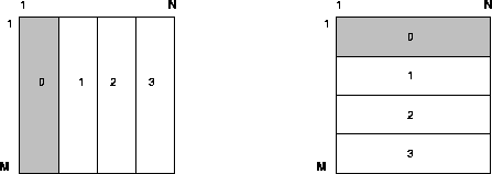
Figure 4.8: The one-dimensional block-column and block-row distributions
assigns a block of NB contiguous
columns of a matrix to successive
processes arranged in a ![]() one-dimensional process grid. Each
process receives at most one block
of columns of the matrix, i.e.,
one-dimensional process grid. Each
process receives at most one block
of columns of the matrix, i.e.,
![]() .
Column k is stored on process
.
Column k is stored on process
![]() .
The maximum number of columns
stored per process is given by
.
The maximum number of columns
stored per process is given by
![]() . In the
figure M=N=16 and P=4.
This distribution assigns
blocks of columns of size
NB to successive processes.
If the value of P evenly
divides the value of
N and NB = N / P, then
each process owns a block of
equal size. However, if this
is not the case, then either
the last process to receive
a portion of the matrix will
receive a smaller block than
other processes, or some
processes may receive an
empty portion of the matrix.
The transpose of this layout,
the one-dimensional
block-row distribution,
is shown on the right of
figure 4.8.
. In the
figure M=N=16 and P=4.
This distribution assigns
blocks of columns of size
NB to successive processes.
If the value of P evenly
divides the value of
N and NB = N / P, then
each process owns a block of
equal size. However, if this
is not the case, then either
the last process to receive
a portion of the matrix will
receive a smaller block than
other processes, or some
processes may receive an
empty portion of the matrix.
The transpose of this layout,
the one-dimensional
block-row distribution,
is shown on the right of
figure 4.8.
The block-column distribution scheme is the data layout that is used in the ScaLAPACK library for the coefficient matrix of the narrow band and tridiagonal solvers.
The block-row distribution scheme is the data layout that is used in the ScaLAPACK library for the right-hand-side matrix of the narrow band and tridiagonal solvers.