Let A be a square n-by-n matrix. A scalar ![]() is called
an eigenvalue and a nonzero column vector v the corresponding
right eigenvector if
is called
an eigenvalue and a nonzero column vector v the corresponding
right eigenvector if ![]() . A nonzero column vector u
satisfying
. A nonzero column vector u
satisfying ![]() is called the left eigenvector .
The first basic task
of the routines described in this section
is to compute, for a given matrix A, all n values of
is called the left eigenvector .
The first basic task
of the routines described in this section
is to compute, for a given matrix A, all n values of ![]() and,
if desired, their associated right eigenvectors v and/or
left eigenvectors u.
and,
if desired, their associated right eigenvectors v and/or
left eigenvectors u.
A second basic task is to compute the Schur factorization of a matrix A.
If A is complex, then its Schur factorization is ![]() , where
Z is unitary and T is upper triangular. If A is real, its
Schur factorization is
, where
Z is unitary and T is upper triangular. If A is real, its
Schur factorization is ![]() , where Z is orthogonal,
and T is upper quasi-triangular (1-by-1 and 2-by-2 blocks on
its diagonal).
The columns of Z are called the Schur vectors of A.
The eigenvalues of A appear on the diagonal of T; complex conjugate
eigenvalues of a real A correspond to 2-by-2 blocks on the diagonal
of T.
, where Z is orthogonal,
and T is upper quasi-triangular (1-by-1 and 2-by-2 blocks on
its diagonal).
The columns of Z are called the Schur vectors of A.
The eigenvalues of A appear on the diagonal of T; complex conjugate
eigenvalues of a real A correspond to 2-by-2 blocks on the diagonal
of T.
These two basic tasks can be performed in the following stages:
The algorithm used in PxLAHQR is similar to the LAPACK routine xLAHQR. Unlike xLAHQR, however, instead of sending one double shift through the largest unreduced submatrix, this algorithm sends multiple double shifts and spaces them apart so that there can be parallelism across several processor row/columns. Another critical difference is that this algorithm applies multiple double shifts in a block fashion, as opposed to xLAHQR which applies one double shift at a time, and xHSEQR from LAPACK which attempts to achieve a blocked code by combining the double shifts into one single large multi-shift. For complete details, please refer to [79].
See table 3.9 for a complete list of the routines.
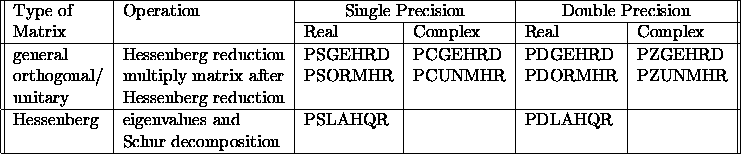
Table 3.9: Computational routines for the nonsymmetric eigenproblem