ScaLAPACK routines return four types of floating-point output arguments:
First, consider scalars. Let the scalar ![]() be an approximation of
the true answer
be an approximation of
the true answer ![]() . We can measure the difference between
. We can measure the difference between ![]() and
and ![]() either by the absolute error
either by the absolute error
![]() , or, if
, or, if ![]() is nonzero, by the relative error
is nonzero, by the relative error
![]() . Alternatively, it is sometimes more convenient
to use
. Alternatively, it is sometimes more convenient
to use ![]() instead of the standard expression
for relative error.
If the relative error of
instead of the standard expression
for relative error.
If the relative error of ![]() is, say,
is, say, ![]() , we say that
, we say that
![]() is accurate to 5 decimal digits.
is accurate to 5 decimal digits.
To measure the error in vectors, we need to measure the size
or norm of a vector x . A popular norm
is the magnitude of the largest component, ![]() ,
which we denote by
,
which we denote by
![]() . This is read the infinity norm of x.
See Table 6.2 for a summary of norms.
. This is read the infinity norm of x.
See Table 6.2 for a summary of norms.
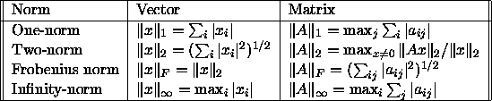
Table 6.2: Vector and matrix norms
If ![]() is an approximation to the
exact vector x, we will refer to
is an approximation to the
exact vector x, we will refer to ![]() as the
absolute error in
as the
absolute error in ![]() (where p is one of the values in Table 6.2)
and refer to
(where p is one of the values in Table 6.2)
and refer to ![]() as the relative error
in
as the relative error
in ![]() (assuming
(assuming ![]() ). As with scalars,
we will sometimes use
). As with scalars,
we will sometimes use ![]() for the relative error.
As above, if the relative error of
for the relative error.
As above, if the relative error of ![]() is, say
is, say ![]() , we say
that
, we say
that ![]() is accurate to 5 decimal digits.
The following example illustrates these ideas.
is accurate to 5 decimal digits.
The following example illustrates these ideas.
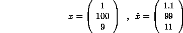
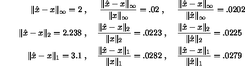
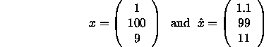
Thus, we would say that ![]() approximates x to 2
decimal digits.
approximates x to 2
decimal digits.
Errors in matrices may also be measured with norms .
The most obvious
generalization of ![]() to matrices would appear to be
to matrices would appear to be
![]() , but this does not have certain
important mathematical properties that make deriving error bounds
convenient.
Instead, we will use
, but this does not have certain
important mathematical properties that make deriving error bounds
convenient.
Instead, we will use
![]() ,
where A is an m-by-n matrix, or
,
where A is an m-by-n matrix, or
![]() ;
see Table 6.2 for other matrix norms.
As before,
;
see Table 6.2 for other matrix norms.
As before, ![]() is the absolute
error
in
is the absolute
error
in ![]() ,
, ![]() is the relative error
in
is the relative error
in ![]() , and a relative error in
, and a relative error in ![]() of
of
![]() means
means ![]() is accurate to 5 decimal digits.
The following example illustrates these ideas.
is accurate to 5 decimal digits.
The following example illustrates these ideas.
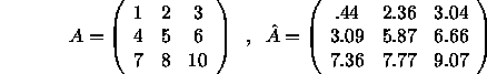
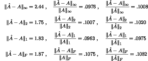
so ![]() is accurate to 1 decimal digit.
is accurate to 1 decimal digit.
We now introduce some related notation we will use in our error bounds.
The condition number of a matrix A is defined as
![]() , where A
is square and invertible, and p is
, where A
is square and invertible, and p is ![]() or one of the other
possibilities in Table 6.2. The condition number
measures how sensitive
or one of the other
possibilities in Table 6.2. The condition number
measures how sensitive ![]() is to changes in A; the larger
the condition number, the more sensitive is
is to changes in A; the larger
the condition number, the more sensitive is ![]() . For example,
for the same A as in the last example,
. For example,
for the same A as in the last example,
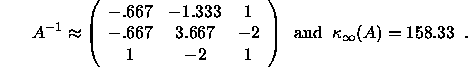
ScaLAPACK
error estimation routines typically compute a variable called
RCOND , which is the reciprocal of the condition number (or an
approximation of the reciprocal). The reciprocal of the condition
number is used instead of the condition number itself in order
to avoid the possibility of overflow when the condition number is very large.
Also, some of our error bounds will use the vector of absolute values
of x, |x| (![]() ), or similarly |A|
(
), or similarly |A|
(![]() ).
).
Now we consider errors in subspaces. Subspaces are the
outputs of routines that compute eigenvectors and invariant
subspaces of matrices. We need a careful definition
of error in these cases for the following reason. The nonzero vector x is called a
(right) eigenvector of the matrix A with eigenvalue
![]() if
if ![]() . From this definition, we see that
-x, 2x, or any other nonzero multiple
. From this definition, we see that
-x, 2x, or any other nonzero multiple ![]() of x is also an
eigenvector. In other words, eigenvectors are not unique. This
means we cannot measure the difference between two supposed eigenvectors
of x is also an
eigenvector. In other words, eigenvectors are not unique. This
means we cannot measure the difference between two supposed eigenvectors
![]() and x by computing
and x by computing ![]() , because this may
be large while
, because this may
be large while ![]() is small or even zero for
some
is small or even zero for
some ![]() . This is true
even if we normalize x so that
. This is true
even if we normalize x so that ![]() , since both
x and -x can be normalized simultaneously. Hence, to define
error in a useful way, we need instead to consider the set
, since both
x and -x can be normalized simultaneously. Hence, to define
error in a useful way, we need instead to consider the set ![]() of
all scalar multiples
of
all scalar multiples ![]() of
x. The set
of
x. The set ![]() is
called the subspace spanned by x and is uniquely determined
by any nonzero member of
is
called the subspace spanned by x and is uniquely determined
by any nonzero member of ![]() . We will measure the difference
between two such sets by the acute angle between them.
Suppose
. We will measure the difference
between two such sets by the acute angle between them.
Suppose ![]() is spanned by
is spanned by ![]() and
and
![]() is spanned by
is spanned by ![]() . Then the acute angle between
. Then the acute angle between
![]() and
and ![]() is defined as
is defined as
![]()
One can show that ![]() does not change when either
does not change when either
![]() or x is multiplied by any nonzero scalar. For example, if
or x is multiplied by any nonzero scalar. For example, if
as above, then ![]() for any
nonzero scalars
for any
nonzero scalars ![]() and
and ![]() .
.
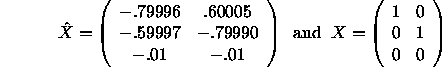
Let us consider another way to interpret the angle ![]() between
between ![]() and
and
![]() .
Suppose
.
Suppose ![]() is a unit vector (
is a unit vector (![]() ).
Then there is a scalar
).
Then there is a scalar ![]() such that
such that
![]()
The approximation ![]() holds when
holds when ![]() is much less than 1
(less than .1 will do nicely). If
is much less than 1
(less than .1 will do nicely). If ![]() is an approximate
eigenvector with error bound
is an approximate
eigenvector with error bound ![]() ,
where x is a true eigenvector, there is another true eigenvector
,
where x is a true eigenvector, there is another true eigenvector
![]() satisfying
satisfying ![]() .
For example, if
.
For example, if
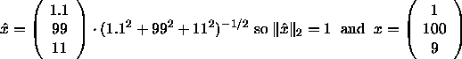
then ![]() for
for
![]() .
.
Finally, many of our error bounds will contain a factor p(n) (or p(m,n)), which grows as a function of matrix dimension n (or dimensions m and n). It represents a potentially different function for each problem. In practice, the true errors usually grow at most linearly; using p(n)=1 in the error bound formulas will often give a reasonable estimate; p(n)=n is more conservative. Therefore, we will refer to p(n) as a ``modestly growing'' function of n; however. it can occasionally be much larger. For simplicity, the error bounds computed by the code fragments in the following sections will use p(n)=1. This means these computed error bounds may occasionally slightly underestimate the true error. For this reason we refer to these computed error bounds as ``approximate error bounds.''
Further Details: How to Measure Errors
The relative error ![]() in the approximation
in the approximation
![]() of the true solution
of the true solution ![]() has a drawback: it often cannot
be computed directly, because it depends on the unknown quantity
has a drawback: it often cannot
be computed directly, because it depends on the unknown quantity
![]() . However, we can often instead estimate
. However, we can often instead estimate
![]() , since
, since ![]() is
known (it is the output of our algorithm). Fortunately, these two
quantities are necessarily close together, provided either one is small,
which is the only time they provide a useful bound anyway. For example,
is
known (it is the output of our algorithm). Fortunately, these two
quantities are necessarily close together, provided either one is small,
which is the only time they provide a useful bound anyway. For example,
![]() implies
implies
![]()
so they can be used interchangeably.
Table 6.2 contains a variety of norms we will use to
measure errors.
These norms have the properties that
![]() , and
, and
![]() , where p is one of
1, 2,
, where p is one of
1, 2, ![]() , and F. These properties are useful for deriving
error bounds.
, and F. These properties are useful for deriving
error bounds.
An error bound that uses a given norm may be changed into an error bound
that uses another norm. This is accomplished by multiplying the first
error bound by an appropriate function of the problem dimension.
Table 6.3 gives the
factors ![]() such that
such that ![]() , where
n is the dimension of x.
, where
n is the dimension of x.
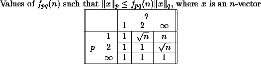
Table 6.3: Bounding one vector norm in terms of another
Table 6.4 gives the
factors ![]() such that
such that ![]() , where
A is m-by-n.
, where
A is m-by-n.
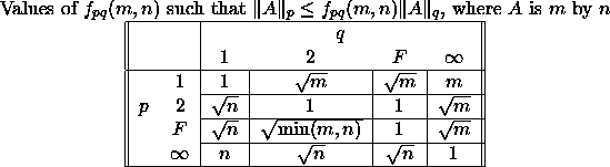
Table 6.4: Bounding one matrix norm in terms of another
The two-norm of A, ![]() , is also called the spectral
norm of A and is equal to the largest singular value
, is also called the spectral
norm of A and is equal to the largest singular value
![]() of A.
We shall also need to refer to the smallest singular value
of A.
We shall also need to refer to the smallest singular value
![]() of A; its value can be defined in a similar way to
the definition of the two-norm in Table 6.2, namely, as
of A; its value can be defined in a similar way to
the definition of the two-norm in Table 6.2, namely, as
![]() when A
has at least as many rows as columns, and defined as
when A
has at least as many rows as columns, and defined as
![]() when A has more
columns than rows. The two-norm,
Frobenius norm ,
and singular values of a matrix do not change
if the matrix is multiplied by a real orthogonal (or complex unitary) matrix.
when A has more
columns than rows. The two-norm,
Frobenius norm ,
and singular values of a matrix do not change
if the matrix is multiplied by a real orthogonal (or complex unitary) matrix.
Now we define subspaces spanned by more than one vector,
and angles between subspaces.
Given a set of k
n-dimensional vectors ![]() , they determine
a subspace
, they determine
a subspace ![]() consisting of all their possible linear combinations
consisting of all their possible linear combinations
![]() ,
, ![]() scalars
scalars ![]() . We also
say that
. We also
say that ![]() spans
spans ![]() .
The difficulty in measuring the difference between subspaces is that
the sets of vectors spanning them are not unique.
For example,
.
The difficulty in measuring the difference between subspaces is that
the sets of vectors spanning them are not unique.
For example, ![]() ,
, ![]() and
and ![]() all determine the
same subspace.
Therefore, we cannot simply compare the subspaces spanned by
all determine the
same subspace.
Therefore, we cannot simply compare the subspaces spanned by
![]() and
and ![]() by
comparing each
by
comparing each ![]() to
to ![]() . Instead, we will measure the angle
between the subspaces, which is independent of the spanning set
of vectors. Suppose subspace
. Instead, we will measure the angle
between the subspaces, which is independent of the spanning set
of vectors. Suppose subspace ![]() is spanned by
is spanned by
![]() and that subspace
and that subspace ![]() is spanned by
is spanned by ![]() . If k=1, we instead write more
simply
. If k=1, we instead write more
simply ![]() and
and ![]() .
When k=1, we define
the angle
.
When k=1, we define
the angle ![]() between
between
![]() and
and ![]() as the acute angle
between
as the acute angle
between ![]() and x.
When k>1, we define the acute angle between
and x.
When k>1, we define the acute angle between ![]() and
and
![]() as the largest acute angle between any vector
as the largest acute angle between any vector ![]() in
in
![]() and the closest vector x in
and the closest vector x in ![]() to
to ![]() :
:
![]()
ScaLAPACK routines that compute subspaces return
vectors ![]() spanning a subspace
spanning a subspace
![]() that are orthonormal. This means the
n-by-k matrix
that are orthonormal. This means the
n-by-k matrix ![]() satisfies
satisfies ![]() . Suppose also that
the vectors
. Suppose also that
the vectors ![]() spanning
spanning ![]() are orthonormal, so
are orthonormal, so ![]() also
satisfies
also
satisfies ![]() .
Then there is a simple expression for the angle between
.
Then there is a simple expression for the angle between
![]() and
and ![]() :
:
![]()
For example, if
then ![]() .
.
As stated above, all our bounds will contain a factor
p(n) (or p(m,n)), which measures how roundoff errors can grow
as a function of matrix dimension n (or m and m).
In practice, the true error usually grows just linearly with n,
or even slower,
but we can generally prove only much weaker bounds of the form ![]() .
This is because we cannot rule out the extremely unlikely possibility of rounding
errors all adding together instead of canceling on average. Using
.
This is because we cannot rule out the extremely unlikely possibility of rounding
errors all adding together instead of canceling on average. Using
![]() would give pessimistic and unrealistic bounds, especially
for large n, so we content ourselves with describing p(n) as a
``modestly growing'' polynomial function of n. Using p(n)=1 in
the error bound formulas will often give a reasonable error estimate.
For detailed derivations of various
p(n), see [71, 114, 84, 38].
would give pessimistic and unrealistic bounds, especially
for large n, so we content ourselves with describing p(n) as a
``modestly growing'' polynomial function of n. Using p(n)=1 in
the error bound formulas will often give a reasonable error estimate.
For detailed derivations of various
p(n), see [71, 114, 84, 38].
There is also one situation where p(n) can grow as large as ![]() :
Gaussian elimination. This typically occurs only on specially constructed
matrices presented in numerical analysis courses [114, p. 212,].
However, the expert driver for solving linear systems, PxGESVX ,
provides error bounds incorporating p(n), and so this rare possibility
can be detected.
:
Gaussian elimination. This typically occurs only on specially constructed
matrices presented in numerical analysis courses [114, p. 212,].
However, the expert driver for solving linear systems, PxGESVX ,
provides error bounds incorporating p(n), and so this rare possibility
can be detected.