Orthogonal Projection Methods.

Let $A$ be an $n \times n$ complex matrix and $\KK$ be an $m$-dimensional subspace of ${\cal C}^n$ and consider the eigenvalue problem of finding $u$ belonging to ${\cal C}^n$ and $\lambda$ belonging to ${\cal C}$ such that

$$A u\ = \ \lambda u .$$ (7)

An orthogonal projection technique onto the subspace $\KK$ seeks an approximate eigenpair $\tilde \lambda , \tlu$ to the above problem, with $\tla$ in ${\cal C}$ and $\tlu$ in $\KK$. This approximate eigenpair is obtained by imposing the following Galerkin condition:

$$A \tlu - \tilde \lambda \tlu \ \bot\ \KK ,$$ (8)

or, equivalently,

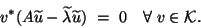$$v^{\ast} ( A \tlu - \tilde \lambda \tlu )\ =\ 0 \ \ \ \forall \ v \in \KK.$$ (9)

In order to translate this into a matrix problem, assume that an orthonormal basis $\{ v_1 , v_2 , \ldots , v_m \}$ of $\KK$ is available. Denote by $V$ the matrix with column vectors $v_1, v_2, \ldots , v_m$, i.e., $V = [v_1, v_2, \ldots , v_m]$. Because we seek a $\tlu \in \KK$, it can be written as

$$\tlu\ =\ V y .$$ (10)

Then, equation eq:4.16 becomes

$$v^{\ast}_j ( A V y - \tilde \lambda V y )= 0 , \quad j=1,\ldots , m .$$

Therefore, $y$ and $\tilde \lambda$ must satisfy

$$B_m y\ =\ \tilde \lambda y$$ (11)

with B_m = V^ A V . The approximate eigenvalues $\tla_i$ resulting from the projection process are all the eigenvalues of the matrix $B_m$. The associated eigenvectors are the vectors $Vy_i$ in which $y_i$ is an eigenvector of $B_m$ associated with $\tla_i$.

This procedure for numerically computing the Galerkin approximations to the eigenvalues/eigenvectors of $A$ is known as the Rayleigh-Ritz procedure.

RAYLEIGH-RITZ PROCEDURE

1. Compute an orthonormal basis $\{ v_i \}_{i=1, \ldots, m}$ of the subspace $\KK$. Let $V = [v_1, v_2, \ldots , v_m]$.
2. Compute $B_m = V^{\ast} A V$.
3. Compute the eigenvalues of $B_m$ and select the $k$ desired ones $\tilde \lambda_i ,i=1,2,\ldots ,k$, where $k \leq m$ (for instance the largest ones).
4. Compute the eigenvectors $y_i , i=1,\ldots ,k$, of $B_m$ associated with $\tilde \lambda_i , i=1,\ldots ,k$, and the corresponding approximate eigenvectors of $A$, $\tlu_i = V y_i , i=1,\ldots ,k$.

In implementations of this approach, one often does not compute the eigenpairs of $B_m$ for each set of generated basis vectors. The values $\tla_i$ computed from this procedure are referred to as Ritz values and the vectors $\tlu_i$ are the associated Ritz vectors. The numerical solution of the $m \times m$ eigenvalue problem in steps 3 and 4 can be treated by standard library subroutines such as those in LAPACK [12]. Another important note is that in step 4 one can replace eigenvectors by Schur vectors to get approximate Schur vectors $\tlu_i$ instead of approximate eigenvectors. Schur vectors $y_i$ can be obtained in a numerically stable way and, in general, eigenvectors are more sensitive to rounding errors than are Schur vectors.