A well-known idea of using simultaneous or block iterations
provides an important improvement over single-vector methods
and permits us to
compute an ![]() -dimensional invariant subspace, rather than one
eigenvector at a time. It can also serve as an acceleration
technique over single-vector methods on parallel computers,
as convergence for extreme eigenvalues usually increases
with the size of the block and every step can be naturally
implemented on wide varieties of multiprocessor computers.
-dimensional invariant subspace, rather than one
eigenvector at a time. It can also serve as an acceleration
technique over single-vector methods on parallel computers,
as convergence for extreme eigenvalues usually increases
with the size of the block and every step can be naturally
implemented on wide varieties of multiprocessor computers.
A block algorithm is a straightforward generalization of the
single-vector
method and is typically combined with the Rayleigh-Ritz
procedure. For every preconditioned eigensolver discussed
earlier, several variants of simultaneous
iterations can be easily suggested; e.g., see
block versions of the preconditioned power method
with shift in [266,149,63,130].
For shortness, we describe here
only one method--a simultaneous version of the locally optimal
PCG method, suggested in [268]--and only
for the pencil ![]() .
.
As in the single-vector algorithm, special measures need to be taken to overcome the problem of almost-linear dependent basis in the trial subspace in Algorithm 11.11.
There is no theory available yet to predict accurately
the speed of convergence of Algorithm 11.11.
However, by analogy with known convergence theory
of PCG system solvers,
we expect convergence of ![]() to
to ![]() to be linear with the ratio
to be linear with the ratio
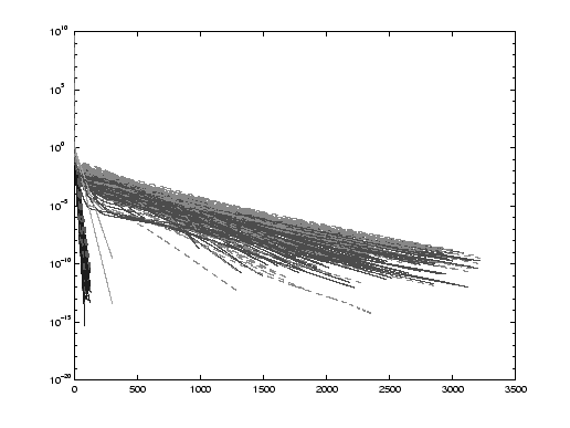
We compared numerically (see [268]) a block variant of the steepest
ascent Algorithm 11.6
and Algorithm 11.11,
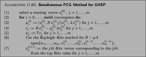
with the block size ![]() . We plot, however, errors for only two top
eigenvalues, leaving the third one out of the picture.
The two shades of red represent the block SA method,
and the two shades of blue correspond to Algorithm 11.11.
It is easy to separate
the methods on a black-and-white print, too,
as Algorithm 11.11 always converges much
faster. Two straight lines correspond to linear
convergence predicted by (11.18).
. We plot, however, errors for only two top
eigenvalues, leaving the third one out of the picture.
The two shades of red represent the block SA method,
and the two shades of blue correspond to Algorithm 11.11.
It is easy to separate
the methods on a black-and-white print, too,
as Algorithm 11.11 always converges much
faster. Two straight lines correspond to linear
convergence predicted by (11.18).
In all tests, ![]() ,
, ![]() is a diagonal matrix with
minimal entries 1, 2, 3 and the maximal entry
is a diagonal matrix with
minimal entries 1, 2, 3 and the maximal entry ![]() and we measure the eigenvalue error as
and we measure the eigenvalue error as
Our random initial guess leads to very big initial errors as the matrix ![]() is
poorly conditioned,
is
poorly conditioned,
![]() . We observe many initial
errors at the level of
. We observe many initial
errors at the level of ![]() on all figures below, but both tested
methods successfully decrease errors to single digits just after
a very few iterations.
on all figures below, but both tested
methods successfully decrease errors to single digits just after
a very few iterations.
We can see that the huge condition number of
![]() , the size of the problem, the distribution of eigenvalues
in the unwanted part of the spectrum, and the
particular choice of the preconditioner
, the size of the problem, the distribution of eigenvalues
in the unwanted part of the spectrum, and the
particular choice of the preconditioner ![]() do not noticeably affect the convergence of
Algorithm 11.11 as
the elements of a bundle, of convergence history lines,
are quite close to each other on all figures.
Moreover, our theoretical prediction (11.18)
of the rate of convergence of Algorithm 11.11
is relatively accurate, though pessimistic.
A 10-fold increase of
do not noticeably affect the convergence of
Algorithm 11.11 as
the elements of a bundle, of convergence history lines,
are quite close to each other on all figures.
Moreover, our theoretical prediction (11.18)
of the rate of convergence of Algorithm 11.11
is relatively accurate, though pessimistic.
A 10-fold increase of
![]() leads to the increase of number of iterations--10-fold
for the block SA method, but only about 3-fold for
Algorithm 11.11--exactly as we would expect.
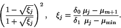
We observe that convergence for the first
eigenvalue, in dark colors, is often faster than
that for the second one, in lighter colors and dashed.
Finally, we also observe a superlinear acceleration when the number of
iterations is
getting comparable with a half of the size of the problem solved.
However, such a large ratio of the number of iterations and the size of
the problem is atypical in practice, so we try to avoid it simply by
increasing the size of the problem; e.g., on Figure 11.3 the
first two runs
are performed for the problem of the size 200; after noticing a
superlinear convergence
we immediately increase the size to 1000.
leads to the increase of number of iterations--10-fold
for the block SA method, but only about 3-fold for
Algorithm 11.11--exactly as we would expect.
We observe that convergence for the first
eigenvalue, in dark colors, is often faster than
that for the second one, in lighter colors and dashed.
Finally, we also observe a superlinear acceleration when the number of
iterations is
getting comparable with a half of the size of the problem solved.
However, such a large ratio of the number of iterations and the size of
the problem is atypical in practice, so we try to avoid it simply by
increasing the size of the problem; e.g., on Figure 11.3 the
first two runs
are performed for the problem of the size 200; after noticing a
superlinear convergence
we immediately increase the size to 1000.
Figures 11.2 to 11.4 clearly illustrate two statements made in §11.1. First, the performance of preconditioned solvers depends heavily on the quality of the preconditioner used. A good preconditioner leads to a fast convergence on Figure 11.2. A bad preconditioner significantly slows the convergence down on Figure 11.4. We note that the size of the problem does not really affect the convergence speed. Second, the implementation particular to each method can make a big difference even with the same preconditioner. This is especially noticeable for poor-quality preconditioners, e.g., on Figure 11.4. Algorithm 11.11, the locally optimal PCG method, converges about a hundred times faster than Algorithm 11.6, though both algorithms use the same preconditioner and have similar costs of every iteration.
To conclude, our numerical results suggest that Algorithm 11.11 is a genuine conjugate gradient method. Our most recent numerical results [269] demonstrate that Algorithm 11.11 is practically the optimal method on the whole class of the preconditioned solvers for symmetric definite eigenvalue problems.
There are known [91] block-preconditioned methods for simultaneous computation of both ends of the spectrum, but they do not offer much improvement over the standard approach of computing minimal and maximal eigenvalues separately.
Another known idea of constructing block eigensolvers
is to use methods of nonlinear optimization
to minimize, or maximize, the trace of
the projection matrix in the Rayleigh-Ritz method (see, e.g.,
[91,16,366] and §9.4), here ![]() .
It leads to methods somewhat similar to Algorithm 11.11
if the conjugate gradient method used for optimization, but Algorithm 11.11 has
an advantage of using the Rayleigh-Ritz method.
.
It leads to methods somewhat similar to Algorithm 11.11
if the conjugate gradient method used for optimization, but Algorithm 11.11 has
an advantage of using the Rayleigh-Ritz method.
The use of locking, a form of deflation, which exploits the unequal convergence rates of the different eigenvectors, enhances the performance of the preconditioned simultaneous iteration methods described above, quite similar to the case of classical methods, without preconditioning; see §4.3. Because of the different rates of convergence of each of the approximate eigenvectors computed by the simultaneous iteration, it is a common practice to extract those already converged and perform a deflation. We freeze extracted approximations and remove them from subsequent iterations such that there is no need to continue to multiply them by any matrices. However, we will still need either to include them in the basis of the trial subspace of the Rayleigh-Ritz method or to perform the subsequent orthogonalizations with respect to the frozen vectors whenever such orthogonalizations are needed.
The former possibility seems more natural and is easier to program than the latter one. It is also quite simple to analyze its influence on the iterative method using known results on accuracy of the Rayleigh-Ritz method; see, e.g., [387,267]. The cost of orthogonalization can be somewhat lower, however, as it reduces the dimension of the trial subspace.
We note that locking should also be used in single-vector iterative methods when we try to compute a group of eigenvectors one by one.
Using orthogonalization for locking in preconditioned eigensolvers may not, unfortunately, be simple if we want to be able to investigate the propagation of the resulting error in the process of further iterations.
As an example, let us consider our simplest
preconditioned eigensolver, Algorithm 11.5,
with additional orthogonalization, defined by an orthogonal
projector ![]() onto an orthogonal complement of the subspace,
spanned by already computed eigenvectors, which can be written as
onto an orthogonal complement of the subspace,
spanned by already computed eigenvectors, which can be written as
First, we need to choose a scalar product for
the orthogonal complement of the subspace,
spanned by already computed eigenvectors. The ![]() -based scalar
seems to be a natural choice here. When
-based scalar
seems to be a natural choice here. When ![]() is positive definite,
it is common to use the
is positive definite,
it is common to use the ![]() -based scalar product as well.
-based scalar product as well.
Second, we need to define a scalar product, in which
projector ![]() is orthogonal. A traditional approach
is to use the same scalar product as on the first step.
It is also trivial to implement in a code.
is orthogonal. A traditional approach
is to use the same scalar product as on the first step.
It is also trivial to implement in a code.
Unfortunately,
with such a choice, the iteration operator in method (11.19)
is loosing the property of being symmetric, with respect to
the ![]() -based scalar product. It makes theoretical investigation of
the influence of orthogonalization to approximately computed
eigenvectors quite complicated (see [147,149]), where direct
analysis of perturbations is done.
-based scalar product. It makes theoretical investigation of
the influence of orthogonalization to approximately computed
eigenvectors quite complicated (see [147,149]), where direct
analysis of perturbations is done.
To preserve the symmetry, we must use the ![]() -orthogonal
projector
-orthogonal
projector ![]() in spite of the fact that we use a different,
say
in spite of the fact that we use a different,
say ![]() -based, scalar product on the first step to define
the orthogonal complement. With this choice, we can use
the standard and simple backward error analysis [264,265]
instead of direct analysis [147,149], but the
actual computation of
-based, scalar product on the first step to define
the orthogonal complement. With this choice, we can use
the standard and simple backward error analysis [264,265]
instead of direct analysis [147,149], but the
actual computation of ![]() for a given
for a given ![]() requires
special attention.
requires
special attention.
Following [264,265], we take the original subspace, spanned by
the frozen approximate
eigenvectors (let us call it ![]() ) and find a
) and find a
![]() -orthogonal basis
of the subspace
-orthogonal basis
of the subspace ![]() . Mathematically, a
. Mathematically, a ![]() -orthogonal
complement to the latter subspace coincides with an
-orthogonal
complement to the latter subspace coincides with an ![]() -orthogonal
complement of the original subspace,
-orthogonal
complement of the original subspace, ![]() . Now, we can
use a standard
. Now, we can
use a standard ![]() -orthogonal projector onto a
-orthogonal projector onto a
![]() -orthogonal complement of
-orthogonal complement of ![]() .
Clearly, the
.
Clearly, the ![]() -based scalar product must be
possible to compute to use this trick.
-based scalar product must be
possible to compute to use this trick.
We also note that the use of a ![]() -based scalar product,
as well as any scalar product based on an ill-conditioned
matrix, may lead to unstable computations.
-based scalar product,
as well as any scalar product based on an ill-conditioned
matrix, may lead to unstable computations.