Transformation to Linear Form

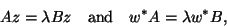
It is easy to see that the QEP in (9.1) is equivalent to the following generalized ``linear'' eigenvalue problem:

$$A z = \lambda B z \quad \mbox{and} \quad w^{\ast} A = \lambda w^{\ast} B ,$$ (248)

where

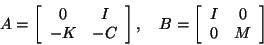$$A = \twobytwo{0}{I}{-K}{-C}, \quad B = \twobytwo{I}{0}{0}{M}$$ (249)

and

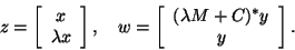$$z = \twobyone{x}{\lambda x}, \quad w = \twobyone{(\lambda M + C)^{\ast} y }{y}.$$ (250)

The generalized eigenvalue problem (9.4) is commonly called a linearization of the QEP (9.1). It can be shown that for any matrices $A$ and $B$ of the above forms, the right and left eigenvectors $z$ and $w$ have the structures described in (9.6).

Note that from the factorization

$$A - \lambda B = \twobytwo{0}{I}{-I}{-\lambda M - C} \twobyt... ... M + \lambda C + K}{0}{0}{I} \twobytwo{I}{0}{-\lambda I }{I},$$ (251)

we can conclude that the pencil $A - \lambda B$ is equivalent to the matrix

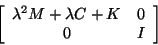$$\twobytwo{\lambda^2 M + \lambda C + K }{0}{0}{I}$$ (252)

and

$${\rm det}(A - \lambda B ) = {\rm det}(\lambda^2 M + \lambda C + K).$$

This means that the eigenvalues of the original QEP (9.1) coincide with the eigenvalues of the generalized eigenvalue problem (9.4). Furthermore, we have that

• $L(\lambda)$ is regular if and only if $A - \lambda B$ is regular;
• if $M$ (hence $B$) is nonsingular, then $L(\lambda)$ is regular;
• if $K$ (hence $A$) is nonsingular, then $L(\lambda)$ is regular.

For the theory on regular pencils $(A,B)$, see, for instance, [425, Chap. VI]. We will assume that at least $M$ is nonsingular throughout this section.

A disadvantage of the above reduction to linear form is that if the matrices $M$, $C$, and $K$ are all Hermitian, then this is not reflected in the reduced form (9.5), where $A$ is non-Hermitian. This can be repaired as follows.

In fact, the matrix pair $(A,B)$ in (9.4) can be chosen in a more general form

$$A = \twobytwo{0}{W}{- K}{ - C}, \quad B = \twobytwo{W}{0}{0}{ M},$$

where $W$ can be any arbitrary nonsingular matrix. Note that now the matrix pencil $A - \lambda B$ is equivalent to the matrix polynomial (9.8) if and only if $W$ is nonsingular, and because of (9.7),

$$\det( A - \lambda B ) = \det(W)\cdot \det( \lambda^2 M + \lambda C + K ).$$

For example, if the matrices $M$, $K$, and $C$ are all symmetric, as in the special case (9.2), and $K$ is nonsingular, then we may choose $W = - K$, which leads to the following symmetric generalized ``linear'' eigenvalue problem

$$A z = \lambda B z \quad \mbox{and} \quad w^{\ast} A = \lambda w^{\ast} B ,$$ (253)

where

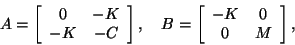$$A = \twobytwo{0}{-K}{-K}{ -C}, \quad B = \twobytwo{-K}{0}{0}{M}, \quad$$ (254)

and

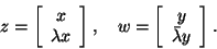$$z = \twobyone{x}{\lambda x}, \quad w = \twobyone{y}{\bar\lambda y}.$$ (255)

Both $A$ and $B$ are symmetric, but may be indefinite.