


Next: Algorithm
Up: Band Lanczos Method
Previous: Deflation
Contents
Index
Basic Properties
After  iterations, the algorithm has generated the
vectors (7.62).
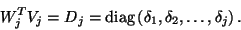
It will be convenient to introduce the notation
iterations, the algorithm has generated the
vectors (7.62).
It will be convenient to introduce the notation
![\begin{displaymath}
V_j = \left[ \begin{array}{cccc}
v_1 & v_2 & \cdots & v_j
...
...in{array}{cccc}
w_1 & w_2 & \cdots & w_j
\end{array} \right]
\end{displaymath}](img2369.png) |
(169) |
for the matrices whose columns are just the right and left Lanczos
vectors (7.62), respectively.
The vectors (7.62) are constructed to be
biorthogonal.
Using the notation (7.63), the biorthogonality can
be stated compactly as follows:
 |
(170) |
In order to enforce biorthogonality of the next Lanczos vectors,
the algorithm involves division by the diagonal entries,  ,
in (7.64).
As a result, the algorithm has to be stopped as soon as
,
in (7.64).
As a result, the algorithm has to be stopped as soon as
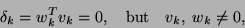 |
(171) |
occurs.
The situation (7.65) is called a breakdown
of the algorithm.
While breakdowns can be remedied by incorporating so-called
look-ahead into the algorithm, here, for simplicity,
we discuss only the band Lanczos algorithm without
look-ahead.
After iterations, in addition to (7.62), the algorithm
has constructed the vectors
 |
(172) |
The vectors
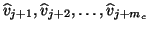 are the candidates for the next
  right Lanczos
vectors,
right Lanczos
vectors,
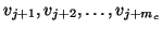 ,
and the vectors
,
and the vectors
 are the candidates for the next
  left Lanczos
vectors,
left Lanczos
vectors,
 .
Here, is the number of right starting vectors,
.
Here, is the number of right starting vectors,  , minus
the number of deflations in the right block Krylov
sequence that have occurred
during the first iterations,
and is the number of left starting vectors,
, minus
the number of deflations in the right block Krylov
sequence that have occurred
during the first iterations,
and is the number of left starting vectors,  , minus
the number of deflations in the left block Krylov
sequence that have occurred
during the first iterations.
The vectors (7.66) are constructed so that they
satisfy the biorthogonality relations
, minus
the number of deflations in the left block Krylov
sequence that have occurred
during the first iterations.
The vectors (7.66) are constructed so that they
satisfy the biorthogonality relations
 |
(173) |
The algorithm has a very simple built-in deflation
procedure based on the vectors (7.66).
In fact, an exact deflation in the right block Krylov
sequence at iteration  is equivalent
to
is equivalent
to
 .
Therefore, in the algorithm, one checks if
.
Therefore, in the algorithm, one checks if
 is smaller than some suitable deflation tolerance.
If yes, the vector
is smaller than some suitable deflation tolerance.
If yes, the vector  is deflated and is
reduced by 1.
Otherwise, is normalized to become the next
right Lanczos vector
is deflated and is
reduced by 1.
Otherwise, is normalized to become the next
right Lanczos vector  .
Similarly, an exact deflation in the left block Krylov
sequence at iteration is equivalent
to
.
Similarly, an exact deflation in the left block Krylov
sequence at iteration is equivalent
to
 .
In the algorithm, one checks if
.
In the algorithm, one checks if
 is smaller than the deflation tolerance.
If yes, the vector
is smaller than the deflation tolerance.
If yes, the vector  is deflated and is
reduced by 1.
Otherwise, is normalized to become the next
left Lanczos vector
is deflated and is
reduced by 1.
Otherwise, is normalized to become the next
left Lanczos vector  .
.
The recurrences that are used in the algorithm to generate the
vectors (7.62) and (7.66) can be summarized
compactly as follows:
![\begin{displaymath}
\begin{array}{rl}
A V_j &\!\!\! = V_j T_j + \left[ \begin{ar...
..._c}
\end{array} \right]
+ \hat{W}_j^{\rm {(dl)}}.
\end{array}\end{displaymath}](img2383.png) |
(174) |
Here,  and
and  are
are  matrices whose entries
are chosen so that the biorthogonality conditions (7.64)
and (7.67) are satisfied.
The matrix
matrices whose entries
are chosen so that the biorthogonality conditions (7.64)
and (7.67) are satisfied.
The matrix
 in (7.68) contains
mostly zero columns, together with the
in (7.68) contains
mostly zero columns, together with the  vectors that have been deflated during the first iterations.
The matrix
vectors that have been deflated during the first iterations.
The matrix
 in (7.68) contains
mostly zero columns, together with the
in (7.68) contains
mostly zero columns, together with the  vectors that have been deflated during the first iterations.
We remark that
vectors that have been deflated during the first iterations.
We remark that  is the number of deflated vectors
and that
is the number of deflated vectors
and that  is the number of deflated vectors.
It turns out that biorthogonality only has to be explicitly enforced
among
is the number of deflated vectors.
It turns out that biorthogonality only has to be explicitly enforced
among  consecutive Lanczos vectors and, once deflation has
occurred, against fixed earlier left Lanczos vectors,
respectively, fixed earlier right Lanczos vectors.
As a result, the matrices and are
``essentially'' banded.
More precisely, has lower bandwidth
consecutive Lanczos vectors and, once deflation has
occurred, against fixed earlier left Lanczos vectors,
respectively, fixed earlier right Lanczos vectors.
As a result, the matrices and are
``essentially'' banded.
More precisely, has lower bandwidth  and
upper bandwidth
and
upper bandwidth  , where the lower bandwidth is reduced by 1
every time a
, where the lower bandwidth is reduced by 1
every time a  vector is deflated, and
the upper bandwidth is reduced by 1
every time a
vector is deflated, and
the upper bandwidth is reduced by 1
every time a  vector is deflated.
In addition, each deflation of a vector
causes to have nonzero elements in a fixed row outside and to
the right of the banded part.
More precisely, the row index of each such row caused by deflation
of a vector is given by
vector is deflated.
In addition, each deflation of a vector
causes to have nonzero elements in a fixed row outside and to
the right of the banded part.
More precisely, the row index of each such row caused by deflation
of a vector is given by  , where
  is the
number of the iteration at which the deflation has occurred
and
is the
number of the iteration at which the deflation has occurred
and  is the corresponding value of at that iteration.
The matrix can thus be written as
is the corresponding value of at that iteration.
The matrix can thus be written as
 |
(175) |
where
 is a banded matrix and
 contains horizontal ``spikes'' above the band of due to
deflation of vectors.
Similarly,
contains horizontal ``spikes'' above the band of due to
deflation of vectors.
Similarly,
where the banded part
 has lower
bandwidth and
upper bandwidth , and
has lower
bandwidth and
upper bandwidth , and
 contains horizontal ``spikes'' above the band of
due to deflation of vectors.
contains horizontal ``spikes'' above the band of
due to deflation of vectors.
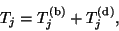
The entries of the matrices and are not
independent of each other.
More precisely, setting
 |
(176) |
we have
 |
(177) |
where  is the diagonal matrix given by (7.64).
Inserting (7.69) into the definition of
is the diagonal matrix given by (7.64).
Inserting (7.69) into the definition of
 in (7.70), we obtain the relation
which shows that
consists of the banded part
,
horizontal spikes due to deflation of vectors
above the banded part, and vertical spikes
due to deflation of vectors
below the banded part.
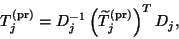
For example, consider the case of  right and
  left
starting vectors.
Assume that during the first
left
starting vectors.
Assume that during the first  iterations, deflations
of vectors have occurred at iterations
iterations, deflations
of vectors have occurred at iterations  ,
,  , and
, and
 , and deflations of vectors have
occurred at iterations
, and deflations of vectors have
occurred at iterations  and
and  .
In this case, the matrix
.
In this case, the matrix
 has the following
sparsity structure:
has the following
sparsity structure:
Here, the  's denote potentially nonzero entries within
the banded part,
's denote potentially nonzero entries within
the banded part,
 ; the
; the  's denote
potentially nonzero entries due to the deflations of
vectors at iterations , , and ;
and the
's denote
potentially nonzero entries due to the deflations of
vectors at iterations , , and ;
and the
 's denote
potentially nonzero entries due to the deflations of
vectors at iterations and .
Note that the deflations have reduced the initial
lower bandwidth
's denote
potentially nonzero entries due to the deflations of
vectors at iterations and .
Note that the deflations have reduced the initial
lower bandwidth  to
to  at iteration
and the initial upper bandwidth
at iteration
and the initial upper bandwidth  to
to  at iteration .
After iterations of the band Lanczos algorithm,
approximate eigensolutions for the NHEP (7.58)
are obtained via an
oblique projection of the matrix  onto the subspace spanned
by the columns of
onto the subspace spanned
by the columns of  and orthogonal to the subspace spanned
by the columns of
and orthogonal to the subspace spanned
by the columns of  .
More precisely, this means that we are seeking approximate
eigenvectors of (7.58) of the form
.
More precisely, this means that we are seeking approximate
eigenvectors of (7.58) of the form
 and that, after inserting this ansatz for
  into (7.58),
we multiply the resulting relation from the left by
into (7.58),
we multiply the resulting relation from the left by  .
This yields the generalized eigenvalue problem
.
This yields the generalized eigenvalue problem
 |
(178) |
Using the biorthogonality relations (7.64)
and (7.67), it is easy to verify that
the matrix
defined in (7.70)
satisfies
 |
(179) |
By (7.73), the generalized eigenvalue
problem (7.72) is equivalent to the standard
eigenvalue problem
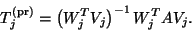
We stress that, in the algorithm, we use the formula in (7.70)
to obtain the entries of
, rather than (7.73).
The band Lanczos algorithm terminates as soon as  or
or  is reached.
In the case , deflations of vectors
have occurred, and thus the right block Krylov
sequence (7.60) is exhausted.
In the case , deflations of vectors
have occurred, and thus the left block Krylov
sequence (7.61) is exhausted.
is reached.
In the case , deflations of vectors
have occurred, and thus the right block Krylov
sequence (7.60) is exhausted.
In the case , deflations of vectors
have occurred, and thus the left block Krylov
sequence (7.61) is exhausted.
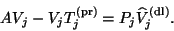
First consider termination due to .
Then, the relation for the
right Lanczos vectors in (7.68) can be rewritten as follows:
 |
(180) |
Here, the matrix
 |
(181) |
represents the oblique projection characterized by
 and
and  for all
  in the null space
of .
Now let
in the null space
of .
Now let
 and
and  be any of the eigenpairs
of
be any of the eigenpairs
of
 , and assume that is normalized
so that
, and assume that is normalized
so that
 .
Recall that the pair
and
is used as an approximate eigensolution
of . From (7.74), it follows that the residual of this
approximate eigensolution can be bounded as follows:
.
Recall that the pair
and
is used as an approximate eigensolution
of . From (7.74), it follows that the residual of this
approximate eigensolution can be bounded as follows:
 |
(182) |
In particular, if only exact deflation is performed, then
 and (7.76) shows that
each eigenvalue
of
is indeed an eigenvalue of .
and (7.76) shows that
each eigenvalue
of
is indeed an eigenvalue of .
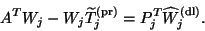
Similarly, in the case of termination due to ,
the relation for the left Lanczos vectors in (7.68)
can be rewritten as follows:
 |
(183) |
Here,  is again the matrix defined in (7.75).
Now let
and
is again the matrix defined in (7.75).
Now let
and
 be any of the
eigenpairs of
be any of the
eigenpairs of
 , and assume that
is normalized such
that
, and assume that
is normalized such
that
 .
Note that the complex conjugate of
is a left
eigenvector of
.
The pair
and
.
Note that the complex conjugate of
is a left
eigenvector of
.
The pair
and
 then represents an approximate eigensolution
of
then represents an approximate eigensolution
of  . From (7.77), it follows that the residual of this
approximate eigensolution can be bounded as follows:
. From (7.77), it follows that the residual of this
approximate eigensolution can be bounded as follows:
 |
(184) |
In particular, if only exact deflation is performed, then
 and (7.78) shows that
each eigenvalue
of
is indeed an eigenvalue of and thus of .
and (7.78) shows that
each eigenvalue
of
is indeed an eigenvalue of and thus of .
Next: Algorithm
Up: Band Lanczos Method
Previous: Deflation
Contents
Index
Susan Blackford
2000-11-20
![\begin{displaymath}
T_{15}^{\rm {(pr)}} = %%\footnotesize{
\left[ \begin{array}{...
...& & & & & &\tilde{{\tt d}}& & & &{*}&{*}
\end{array} \right].
\end{displaymath}](img2403.png)