Basic Algorithm

The Arnoldi method is an orthogonal projection method onto a Krylov subspace. It starts with the Arnoldi procedure as described in Algorithm 7.3. The procedure can be essentially viewed as a modified Gram-Schmidt process for building an orthogonal basis of the Krylov subspace $\KK^m(A,v)$.

The above procedure will stop if the vector $w$ computed in line (8) vanishes. The vectors $v_1, v_2, \ldots , v_m$ form an orthonormal system by construction and are called Arnoldi vectors. An easy induction argument shows that this system is a basis of the Krylov subspace $\KK^m(A,v)$.

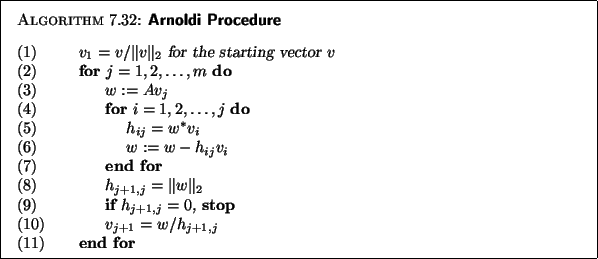
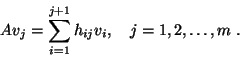
Next we consider a fundamental relation between quantities generated by the algorithm. The following equality is readily derived:

$$A v_j = \sum_{i=1}^{j+1} h_{ij} v_i , \quad j=1,2,\ldots ,m \ .$$ (122)

If we denote by $V_m$ the $n \times m$ matrix with column vectors $v_1, \ldots, v_m$, and by $H_m$ the $m \times m$ Hessenberg matrix whose nonzero entries $h_{ij}$ are defined by the algorithm, then the following relations hold:

$$A V_m = V_m H_m + h_{m+1,m} v_{m+1} e_m^{\ast},$$ (123)

$$V_m^{\ast} A V_m = H_m \ .$$ (124)

Relation eq:VmTAVm follows from eq:AVm by multiplying both sides of eq:AVm by $V_m^{\ast}$ and making use of the orthonormality of $\{ v_1, \ldots,v_m \}$.

As was noted earlier the algorithm breaks down when the norm of $w$ computed on line (8) vanishes at a certain step $j$. As it turns out, this happens if and only if the starting vector $v$ is a combination of $j$ eigenvectors (i.e., the minimal polynomial of $v_1$ is of degree $j$). In addition, the subspace $\KK_j$ is then invariant and the approximate eigenvalues and eigenvectors are exact [387].

The approximate eigenvalues $\lambda_i \sup{m}$ provided by the projection process onto $\KK_m$ are the eigenvalues of the Hessenberg matrix $H_m$. These are known as Ritz values. A Ritz approximate eigenvector associated with a Ritz value $\lambda_i \sup{m}$ is defined by $u_i \sup{m}= V_m y_i \sup{m}$, where $y_i \sup{m}$ is an eigenvector associated with the eigenvalue $\lambda_i \sup{m}$. A number of the Ritz eigenvalues, typically a small fraction of $m$, will usually constitute good approximations for corresponding eigenvalues $\lambda_i$ of $A$, and the quality of the approximation will usually improve as $m$ increases.

The original algorithm consists of increasing $m$ until all desired eigenvalues of $A$ are found. For large matrices, this becomes costly both in terms of computation and storage. In terms of storage, we need to keep $m$ vectors of length $n$ plus an $m \times m$ Hessenberg matrix, a total of approximately $n m + m ^2 /2$. For the arithmetic costs, we need to multiply $v_j$ by $A$, at the cost of $2 \times N_z$, where $N_z$ is number of nonzero elements in $A$, and then orthogonalize the result against $j$ vectors at the cost of $4 (j+1) n,$ which increases with the step number $j$. Thus an $m$-dimensional Arnoldi procedure costs $\approx n m + m ^2 /2$ in storage and $\approx N_z + 2 n m ^2$ in arithmetic operations.

Obtaining the residual norm, for a Ritz pair, as the algorithm progresses is fairly inexpensive. Let $y_i \sup{m}$ be an eigenvector of $H_m$ associated with the eigenvalue $\lambda_i \sup{m}$, and let $u_i \sup{m}$ be the Ritz approximate eigenvector $u_i \sup{m}= V_m y_i \sup{m}$. We have the relation

$$(A - \lambda_i \sup{m}I ) u_i \sup{m}= h_{m+1,m}(e_m^{\ast} y_i\sup{m})v_{m+1},$$

and, therefore,

$$\Vert ( A - \lambda_i \sup{m}I ) u_i \sup{m}\Vert _2 = h_{m+1,m} \vert e_m^{\ast} y_i \sup{m}\vert \ .$$

Thus, the residual norm is equal to the absolute value of the last component of the eigenvector $y_i \sup{m}$ multiplied by $h_{m+1,m}$. The residual norms are not always indicative of actual errors in $\lambda_i \sup{m}$, but can be quite helpful in deriving stopping procedures.