Algorithm

A complete statement of the band Lanczos algorithm for Hermitian matrices $A$ is as follows.

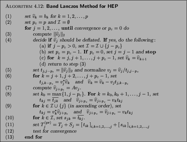
Next, we discuss some of the steps of Algorithm 4.12 in more detail.

(4)

Generally, the decision on whether $\hat{v}_j$ needs to be deflated should be based on checking whether

$$\Vert\hat{v}_j\Vert _2 \leq {\tt dtol},$$ (51)

where ${\tt dtol}$ is a suitably chosen deflation tolerance. The vector $\hat{v}_j$ is then deflated if (4.42) is satisfied. In this case, the value $j-p_c$, if positive, is added to the index set ${\cal I}$, which contains the indices of the nonzero rows in the part $T_j^{\rm {(d)}}$ of $T_j$, and the current block size is updated to $p_c=p_c-1$. If $p_c=0$, the block Krylov sequence (4.27) is exhausted, and the algorithm terminates naturally. If $p_c>0$, the vector $\hat{v_j}$ is deleted, the index $k+1$ of each of the remaining candidate vectors $\hat{v}_{k+1}$ is reset to $k$, and finally, the algorithm returns to step (3). If (4.42) is not satisfied, no deflation is necessary and the algorithm proceeds with step (5).

Usually, in (4.42), one will choose a small tolerance ${\tt dtol}$, such as the square root of machine precision. However, ${\tt dtol}$ does not have to be small; Algorithm 4.12 and its properties remain correct for any choice of ${\tt dtol}$. Note that the algorithm performs only exact deflation if one sets ${\tt dtol}=0$ in (4.42).

(5)

The vector $\hat{v}_j$ has passed the deflation check and is now normalized to become the next Lanczos vector $v_j$. The normalization is such that

$$\left\Vert v_j \right\Vert _2 = 1\quad \mbox{for all}\quad j.$$

(6)

The remaining candidate vectors, $\hat{v}_{j+1},\hat{v}_{j+2},\ldots,\hat{v}_{j+p_c-1}$, are explicitly orthogonalized against the latest Lanczos vector $v_j$. Note that in the first $p$ steps some $t_{j,k-p_c}$ will have nonpositive column index. They serve to make the starting basis orthonormal, but need not be stored in the $T_j$ matrix.

(7)

The block Krylov sequence is advanced by computing a new candidate vector, $\hat{v}_{j+p_c}$, as the $A$-multiple of the latest Lanczos vector $v_j$.

(8)

The vector $\hat{v}_{j+p_c}$ is orthogonalized against the previous Lanczos vectors $v_{k_0}$, $v_{k_0+1}$, $\ldots$, $v_{j-1}$, where $k_0=\max\{1,j-p_c\}$. Here, we exploit the fact that the matrix $T_j^{(\rm pr)}$ is Hermitian, and instead of explicitly computing $t_{kj}$, we set $t_{kj} = \overline{t_{jk}}$. Note that the $t_{jk}$'s were computed explicitly in step (6).

(9)

The vector $\hat{v}_{j+p_c}$ is explicitly orthogonalized against the Lanczos vectors $v_k$, $k\in {\cal I}$, and against $v_j$. Note that modified Gram-Schmidt is used to do this orthogonalization.

(11)

All the nonzero elements in the $j$th row and the $j$th column have now been computed, and they are added to the matrix $T_{j-1}^{(\rm pr)}$ of the previous iteration $j-1$, to yield the current matrix $T_{j}^{(\rm pr)}$. Here, we use the convention that entries $t_{ik}$ and $s_{ik}$ that are not explicitly defined in Algorithm 4.12 are set to zero.

(12)

To test for convergence, the eigenvalues $\theta_i^{(j)}$, $i=1,2,\ldots,j$, of the Hermitian $j\times j$ matrix $T_j^{\rm {(pr)}}$ are computed, and the algorithm is stopped if some of the $\theta_i^{(j)}$'s are good enough approximations to the desired eigenvalues of $A$.