Stability of $Q^* T Q$.

The deflating orthogonal transformation construction shown in Algorithm 4.9 is clearly stable (i.e., a componentwise relatively accurate representation of the transformation one would obtain in exact arithmetic). There is no question that the similarity transformation $Q^* T Q$ preserves the eigenvalues of $T$ to full numerical accuracy. However, there is a serious question about how well the tridiagonal form is preserved during locking and/or purging. A modification to the basic algorithm is needed to assure that if $T y = y \theta$, then $T_+ \equiv Q^* T Q$ is symmetric and numerically tridiagonal (i.e., the entries outside the tridiagonal band are all tiny relative to $\Vert T \Vert$).

The fact that $T_+ = Q^* T Q$ is tridiagonal depends upon the term $g y^* T R$ vanishing in the expression

$$Q^* T Q = L^*TR + g y^*T R + \theta e_1 e_1^*.$$

However, on closer examination, we see that

$$e_1^* Q = e_1^* L + (e_1^* y) g^* = \eta_1 g^*,$$

where $\eta_1$ is the first component of $y$. Therefore, $\Vert g \Vert = \frac{1}{\vert \eta_1 \vert}$. So there may be numerical difficulty when the first component of $y$ is small. To be specific, $y^* T = \theta y^*$ and thus $y^* T R = 0$ in exact arithmetic. However, in finite precision, the computed $\mathrm{fl}(y^* T) = \theta y^* + z^*$. The error $z$ will be on the order of $\epsilon_M$ relative to $\Vert T \Vert$, but

$$\Vert g y^*T R \Vert = \Vert g\Vert \cdot \Vert z^* R \Vert = \frac{1}{\vert \eta_1 \vert} \Vert z^* R \Vert,$$

so this term may be quite large. It may be as large as order $O(1)$ if $\eta_1 = O(\epsilon_M)$. This is of serious concern and will occur in practice without the modification we now propose.

The remedy is to introduce a step-by-step acceptable perturbation and rescaling of the vector $y$ to simultaneously force the conditions

$$Q^* y = e_1 \ \ \mbox{and} \ \ y^* T Q = \theta e_1^*$$

to hold with sufficient accuracy in finite precision. To accomplish this, we shall devise a scheme to achieve

$$y^* T q_j = 0 \ \ \mbox{for} \ \ j > 1$$

numerically. As shown in [420], this modification is sufficient to establish $q_i^* T q_j = 0$ numerically, relative to $\Vert T \Vert$ for $i > j + 1$.

The basic idea is as follows: If, at the $j$th step, the computed quantity $\mathrm{fl}(y^* T q_j )$ is not sufficiently small, it is adjusted to be small enough by scaling the vector $y_j$ with a number $\phi$ and the component $\eta_{j+1}$ with a number $\psi$. With this rescaling just prior to the computation of $q_{j+1}$, we have $y_j \leftarrow y_j \phi$ and $\hat{y}_j \leftarrow \hat{y}_j \psi$, where $y^* = [ y_j^* , \hat{y}_j^*]$. Certainly, $\Vert y \Vert$ should not be altered with this scaling and this is therefore required. This gives the following system of equations to determine $\phi$ and $\psi$: If $\vert y_j^* T_j \hat{q}_j + \rho_j \beta_j \eta_{j+1} \vert > \epsilon_M \tau_{j+1}$, (_j )^2 + (1 - _j^2)^2 &=& 1,
y_j^* T_j q_j + _j _j _j+1 &=& _M _j+1.

If $\rho_j$ is on the order of $\sqrt{\epsilon_M}$, the scaling may be absorbed into $\rho_j$ without alteration of $y$ and also without affecting the numerical orthogonality of $Q$. When $y$ is modified, it turns out that none of the previously computed $q_i, 2 \le i < j,$ need to be altered. After step $j$, the vector $y_j$ is simply rescaled in subsequent steps, and the formulas defining $q_i, 2 \le i \le j,$ are invariant with respect to scaling of $y_j$. For complete detail, one should consult  [420].

Algorithm 4.10 implements this scheme to compute an acceptable $Q$.In practice, this transformation may be computed and applied in place to obtain a $T \leftarrow Q^* T Q$ and $V \leftarrow VQ$ without storing $Q$. However, that implementation is quite subtle and the construction of $Q$ is obscured by the details required to avoid additional storage. This code departs slightly from the above description since the vector $y$ is rescaled to have unit norm only after all of the columns $2$ to $m$ have been determined.

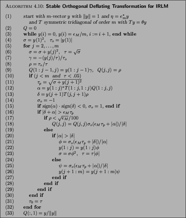
There are several implementation issues.

(3)

The perturbation $y(i)$ shown here avoids problems with exact zero initial entries in the eigenvector $y$. In theory, this should not happen when $T$ is unreduced but it may happen numerically if $\theta$ is weakly represented in the starting vector. There is a cleaner implementation possible that does not modify zero entries. This is the simplest (and crudest) correction.

(10)

As soon as $\tau_j = \Vert y_j\Vert$ is sufficiently large, there is no need for any further corrections. Deleting this if-clause reverts to the unmodified calculation of $Q$ shown in Algorithm 4.9.

(16)

This shows one of several possibilities for modifying $y$ to achieve the desired goal of numerically tiny elements outside the tridiagonal band of $Q^* T Q$. More sophisticated strategies would absorb as much of the scaling as possible into the diagonal element $Q(j,j) = \rho$. Here, the branch that does scale $\rho$ instead of $y$ is designed so that ${\rm fl}(1 + (\rho \psi)^2) = {\rm fl}(1 + \rho^2) = 1$.