We shall use the following example to illustrate the material introduced so far, and to motivate new functions.
Example 2.11 Jacobi iteration - sequential code
REAL A(0:n+1,0:n+1), B(1:n,1:n)
...
!Main Loop
DO WHILE(.NOT.converged)
   ! perform 4 point stencil
   DO j=1, n
      DO i=1, n
         B(i,j)=0.25*(A(i-1,j)+A(i+1,j)+A(i,j-1)+A(i,j+1))
      END DO
   END DO

   ! copy result back into array A
   DO j=1, n
      DO i=1, n
         A(i,j) = B(i,j)
      END DO
   END DO
...
! convergence test omitted
END DO
The code fragment describes the main loop of an iterative solver where
,at each iteration, the value at a point is replaced by the average of
the North , South, East and West neighbours(a fout point pencil is used
to keep example simple).Boundary values do not change.We focus on the
inner loop, where most of the computation is done, and use fortran 90
syntax, for clarity.
Since this code has a simple structure, a data-parallel approach can be
used to derive an equivalent parallel code. The array is distributed
across processes, and each process is assigned the task of updating
the entries on the part of the array it owns.
A parallel
algorithm is derived from a choice of data distribution. The
data distribution
distribution should be balanced, allocating (roughly) the same number
of entries to each processor; and it should minimize communication.
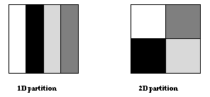
Figure ![]() illustrates two possible distributions: a
1D (block) distribution, where the matrix is partitioned in one dimension,
and a 2D (block,block) distribution, where the matrix is partitioned
in two dimensions.
illustrates two possible distributions: a
1D (block) distribution, where the matrix is partitioned in one dimension,
and a 2D (block,block) distribution, where the matrix is partitioned
in two dimensions.

Figure: Block partitioning of a matrix.
Since the communication occurs at block boundaries, communication volume is minimized by the 2D partition which has a better area to perimeter ratio. However, in this partition, each processor communicates with four neighbors, rather than two neighbors in the 1D partition. When the ratio of n/P (P number of processors) is small, communication time will be dominated by the fixed overhead per message, and the first partition will lead to better performance. When the ratio is large, the second partition will result in better performance. In order to keep the example simple, we shall use the first partition; a realistic code would use a ``polyalgorithm'' that selects one of the two partitions, according to problem size, number of processors, and communication performance parameters.
The value of each point in the array B is computed from the value of the four neighbors in array A. Communications are needed at block boundaries in order to receive values of neighbor points which are owned by another processor. Communications are simplified if an overlap area is allocated at each processor for storing the values to be received from the neighbor processor. Essentially, storage is allocated for each entry both at the producer and at the consumer of that entry. If an entry is produced by one processor and consumed by another, then storage is allocated for this entry at both processors. With such scheme there is no need for dynamic allocation of communication buffers, and the location of each variable is fixed. Such scheme works whenever the data dependencies in the computation are fixed and simple. In our case, they are described by a four point stencil. Therefore, a one-column overlap is needed, for a 1D partition.
We shall partition array A with one column
overlap. No such overlap is required for array B.
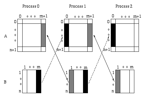
Figure ![]() shows the extra columns in A and
how data is transfered for each iteration.
shows the extra columns in A and
how data is transfered for each iteration.
We shall use an algorithm where all values needed from a neighbor are brought in one message. Coalescing of communications in this manner reduces the number of messages and generally improves performance.

Figure: 1D block partitioning with overlap and communication
pattern for jacobi iteration.
The resulting parallel algorithm is shown below.
Example2.12 Jacobi iteration - first version of parallel code
...
REAL, ALLOCATABLE A(:,:), B(:,:)
...
! Compute number of processes and myrank
CALL MPI_COMM_SIZE(comm, p, ierr)
CALL MPI_COMM_RANK(comm, myrank, ierr)

! compute size of local block
m = n/p
IF (myrank.LT.(n-p*m)) THEN
   m = m+1
END IF

!Allocate local arrays
ALLOCATE (A(0:n+1,0:m+1), B(n,m))
...
!Main Loop
DO WHILE(.NOT.converged)
   ! compute
   DO j=1, m
      DO i=1, n
         B(i,j)=0.25*(A(i-1,j)+A(i+1,j)+A(i,j-1)+A(i,j+1))
      END DO
   END DO

   DO j=1, m
      DO i=1, n
         A(i,j) = B(i,j)
      END DO
   END DO

  ! Communicate
  IF (myrank.GT.0) THEn
      CALL MPI_SEND(B(1,1),n, MPI_REAL, myrank-1, tag, comm, ierr)
      CALL MPI_RECV(A(1,0),n, MPI_REAL, myrank-1, tag, comm,
                                                  status, ierr)
  END IF
  IF (myrank.LT.p-1) THEN
      CALL MPI_SEND(B(1,m),n, MPI_REAL, myrank+1, tag, comm, ierr)
      CALL MPI_RECV(A(1,m+1),n, MPI_REAL, myrank+1, tag, comm,
                                                  status, ierr)
  END IF
...
One way to get a safe version of this code is to
alternate
the order of sends and receives: odd rank processes will first send, next
receive, and even rank processes will first receive, next send. Thus,
one achieves the communication pattern of Example The modified main loop is shown below. We shall later see simpler ways of dealing with this problem. Jacobi, safe version
Example2.13 Main Loop of Jacobi iteration-safe version of parallel code
...
!Main Loop
DO WHILE(.NOT.converged)
   ! compute
   DO j=1, m
      DO i=1, n
         B(i,j)=0.25*(A(i-1,j)+A(i+1,j)+A(i,j-1)+A(i,j+1))
      END DO
   END DO

   DO j=1, m
      DO i=1, n
         A(i,j) = B(i,j)
      END DO
   END DO

  ! Communicate
  IF (MOD(myrank,2).EQ.1)THEN
      CALL MPI_SEND(B(1,1),n, MPI_REAL, myrank-1, tag, comm, ierr)
      CALL MPI_RECV(A(1,0),n, MPI_REAL, myrank-1, tag, comm,
                                                  status, ierr)

     IF (myrank.LT.p-1) THEN
      CALL MPI_SEND(B(1,m),n, MPI_REAL, myrank+1, tag, comm, ierr)
      CALL MPI_RECV(A(1,m+1),n, MPI_REAL, myrank+1, tag, comm,
                                                  status, ierr)
  END IF
  ELSE IF !myrank is even
  IF (myrank.GT.0) THEN
      CALL MPI_RECV(A(1,0),n, MPI_REAL, myrank-1, tag, comm,
                                                  status, ierr)
      CALL MPI_SEND(B(1,1),n, MPI_REAL, myrank-1, tag, comm, ierr)
 END IF
 IF (myrank.LT.p-1) THEN
      CALL MPI_RECV(A(1,m+1),n, MPI_REAL, myrank+1, tag, comm,
                                                  status, ierr)
      CALL MPI_SEND(B(1,m),n, MPI_REAL, myrank+1, tag, comm, ierr)
  END IF
END IF
...
END DO