

Next: The Broyden-Fletcher-Goldfarb-Shanno
One-StepMemoryless
Up: Optimization Methods
for
Previous: 9.9.1 Deficiencies of Steepest
There are no general prescriptions for selecting an appropriate
learning rate  in back-propagation, in order
to avoid oscillations and converge to a good local minimum of the
energy in a short time. In many applications, some kind of ``black
magic,'' or trial-and-error process, is employed. In addition, usually
no fixed learning rate is appropriate for the entire learning
session.
Both problems can be solved by adapting the learning rate to the local
structure of the energy surface.
We start with a given learning rate (the value does not matter) and
monitor the energy after each weight update. If the energy decreases,
the learning rate for the next iteration is increased by a factor
 . Conversely, if the energy increases (an ``accident'' during
learning), this is taken as an indication that the step made was too
long, the learning rate is decreased by a factor
  , the last
change is cancelled, and a new trial is done. The process of reduction
is repeated until a step that decreases the energy value is found (this
will inevitably happen because the search direction is that of the
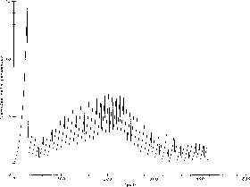
negative gradient). An example of the size of the learning rate as a
function of the iteration number is shown in Figure 9.24.

Figure 9.24: Learning Rate Magnitude as a Function of the Iteration Number for a
Test Problem
The name ``Bold Driver'' was selected for the
analogy with the learning process of young and inexperienced car drivers.
By using this ``brutally heuristic'' method, learning converges in a time
that is comparable to, and usually better than that of standard (batch)
back-propagation with an optimal and fixed learning rate. The
important difference is that the time-consuming meta-optimization
phase for choosing  is avoided. The values for
  and
and  can be fixed once and for all (e.g.,
  ,
,  )
and performance does not depend critically on their choice.


Next: The Broyden-Fletcher-Goldfarb-Shanno
One-StepMemoryless
Up: Optimization Methods
for
Previous: 9.9.1 Deficiencies of Steepest
Guy Robinson
Wed Mar 1 10:19:35 EST 1995
 in back-propagation, in order
to avoid oscillations and converge to a good local minimum of the
energy in a short time. In many applications, some kind of ``black
magic,'' or trial-and-error process, is employed. In addition, usually
no fixed learning rate is appropriate for the entire learning
session.


 . Conversely, if the energy increases (an ``accident'' during
learning), this is taken as an indication that the step made was too
long, the learning rate is decreased by a factor
  , the last
change is cancelled, and a new trial is done. The process of reduction
is repeated until a step that decreases the energy value is found (this
will inevitably happen because the search direction is that of the
negative gradient). An example of the size of the learning rate as a
function of the iteration number is shown in Figure
 is avoided. The values for
  and
and  can be fixed once and for all (e.g.,
  ,
,  )
and performance does not depend critically on their choice.