


Next: Example 11.2.2.
Up: Davidson Method
Previous: Davidson Method
Contents
Index
Here  is symmetric and roughly models matrices from quantum
chemistry.
is symmetric and roughly models matrices from quantum
chemistry.  is the identity matrix. The main diagonal of has
elements
is the identity matrix. The main diagonal of has
elements
 and the off-diagonal elements of the
upper
triangular portion are selected randomly from the interval
and the off-diagonal elements of the
upper
triangular portion are selected randomly from the interval  . We consider computing the smallest eigenvalue of using the diagonal
preconditioning of the original Davidson method. The eigenvalues
of are
. We consider computing the smallest eigenvalue of using the diagonal
preconditioning of the original Davidson method. The eigenvalues
of are  , 0.721, 1.73, 2.77,
  , 101.58. So we let
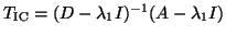
 . The eigenvalues of
 are 0.0, 0.263, 0.387, 0.500, , 2.01. The eigenvalue
  of
of
 is much better separated relative to the entire spectrum than is
 of . In fact, the gap ratio of for is
 , while
the gap ratio for the eigenvalue
, while
the gap ratio for the eigenvalue  of
is
of
is  . With gap ratio
16 times larger, asymptotic convergence is very roughly four times
faster.
The next example looks at a matrix that is tougher to precondition. Some
results can be given similar to those for preconditioning linear
equations.
. With gap ratio
16 times larger, asymptotic convergence is very roughly four times
faster.
The next example looks at a matrix that is tougher to precondition. Some
results can be given similar to those for preconditioning linear
equations.
Susan Blackford
2000-11-20